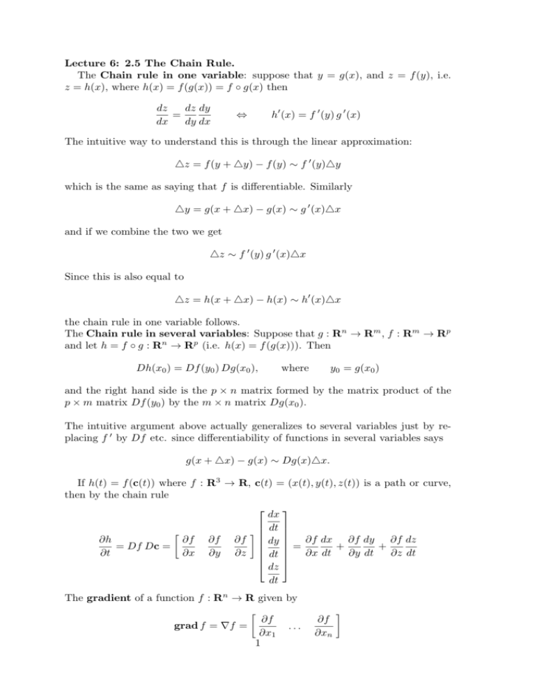
Lecture 6: 2.5 The Chain Rule.
The Chain rule in one variable: suppose that y = g(x), and z = f (y), i.e.
z = h(x), where h(x) = f (g(x)) = f ◦ g(x) then
dz
dz dy
=
dx
dy dx
⇔
h′ (x) = f ′ (y) g ′ (x)
The intuitive way to understand this is through the linear approximation:
△z = f (y + △y) − f (y) ∼ f ′ (y)△y
which is the same as saying that f is differentiable. Similarly
△y = g(x + △x) − g(x) ∼ g ′ (x)△x
and if we combine the two we get
△z ∼ f ′ (y) g ′ (x)△x
Since this is also equal to
△z = h(x + △x) − h(x) ∼ h′ (x)△x
the chain rule in one variable follows.
The Chain rule in several variables: Suppose that g : Rn → Rm , f : Rm → Rp
and let h = f ◦ g : Rn → Rp (i.e. h(x) = f (g(x))). Then
Dh(x0 ) = Df (y0 ) Dg(x0 ),
where
y0 = g(x0 )
and the right hand side is the p × n matrix formed by the matrix product of the
p × m matrix Df (y0 ) by the m × n matrix Dg(x0 ).
The intuitive argument above actually generalizes to several variables just by replacing f ′ by Df etc. since differentiability of functions in several variables says
g(x + △x) − g(x) ∼ Dg(x)△x.
If h(t) = f (c(t)) where f : R3 → R, c(t) = (x(t), y(t), z(t)) is a path or curve,
then by the chain rule


dx


[
]  dt 

∂f ∂f ∂f 
∂h
 dy  = ∂f dx + ∂f dy + ∂f dz
= Df Dc =

∂x ∂y ∂z  dt 
∂t
∂y dt
∂z dt
 ∂x dt
 dz 
dt
The gradient of a function f : Rn → R given by
[
∂f
grad f = ∇f =
...
∂x1
1
∂f
∂xn
]
2
This can also be expressed with the gradient notation and dot product
dh
(t) = ∇f (c(t)) · c ′ (t)
dt
where
c′ (t) = (x′ (t), y ′ (t), z ′ (t)),
is the velocity vector of the path.
Note that c′ (t) is tangent to the path c(t), which follows since it can be obtained
as the limit as h → 0 of the vector between two close points on the curve
c(t+ h) − c(t) ( x(t+ h) − x(t) y(t+ h) − y(t) z(t+ h) − z(t) )
=
,
,
→ (x′ (t), y ′ (t), z ′ (t))
h
h
h
h
Ex. If z = x2 + y 2 , x = cos t and y = sin t find dz/dt.
dz
∂z dx ∂z dy
Sol. 1
=
+
= 2x (− sin t)+2y cos t = 2 cos t (− sin t)+2 sin t cos t = 0
dt
∂x dt ∂y dt
dz
Sol. 2
z = x2 + y 2 = cos2 t + sin2 t = 1,
=0
dt
Ex. If z = h(r, θ) = f (x, y) where x = g1 (r, θ) = r cos θ and y = g2 (r, θ) = r sin θ
then by the chain rule
 ∂g
∂g1 
1
( ∂h ∂h ) ( ∂f ∂f )  ∂r
∂θ 
,
=
,


∂r ∂θ
∂x ∂y
∂g2 ∂g2
∂r
∂θ
i.e.
∂h
∂f ∂x ∂f ∂y
=
+
∂r
∂x ∂r
∂y ∂r
∂h
∂f ∂x ∂f ∂y
=
+
∂θ
∂x ∂θ
∂y ∂θ
or written shorter since h and f is the same function expressed in different coordinates
∂
∂x ∂
∂y ∂
=
+
∂r
∂r ∂x ∂r ∂y
∂x ∂
∂y ∂
∂
=
+
∂θ
∂θ ∂x ∂θ ∂y
In this case the matrix
 ∂x ∂x 
(
)
cos θ −r sin θ
 ∂r ∂θ 

=
sin θ r cos θ
∂y ∂y
∂r ∂θ
∂r
∂x
Note that in general
̸= ( )−1 . whereas for a function of one variable its
∂x
∂r
true that dx/dy = (dy/x)−1 . That this is true in one dimension follows from
differentiating the identity f (f −1 (x)) = x which gives f ′ (f −1 (x))f −1 (x) ′ = 1. The
higher dimension analogue of this would be with the derivative matrices so
 

∂r ∂r
∂x ∂x −1
(
)
 ∂x ∂y   ∂r ∂θ 
1 r cos θ r sin θ
=

 =
 ∂θ ∂θ 
r − sin θ − cos θ
∂y ∂y
∂x ∂y
∂r ∂θ
3
2.6 The gradient and directional derivative.
The gradient of a function f : R3 → R is the vector
(
)
∂f ∂f ∂f
∇f =
,
,
∂x ∂y ∂z
i.e. it is the matrix of derivatives written as a vector.
Consider the equation of a line in space ℓ(t) = x + tv, −∞ < t < ∞.
The function h(t) = f◦ ℓ(t) = f (x + tv) represents the function f restricted to the line.
The directional derivative of f at x in the direction of unit vector v is given by
d
= ∇f (x) · v
f (x + tv)
dt
t=0
Here the equality follows from the chain rule: h ′ = Dh = Df Dℓ = ∇f · ℓ ′ = ∇f · v.
The reason we choose v to be a unit vector is that we want the directional derivative
to represent the rate of change in different directions.
Suppose that f represents the temperature at different points in space. Suppose
that a fly flies along the line above at unit speed then the change of temperature
per unit time or distance is the directional derivative.
The gradient points in the direction along which f increases the fastest.
In fact ∇f · v = |∇f | |v| cos θ, where θ is the angle between ∇f and v, and the
max is when cos θ = 1.
Suppose we are lost in wood and we want to reach a high hill top to see where we
are. However, we can only see a few feet in front of us because of the high trees.
In which direction shall we go in order to reach a hill-top fast. The answer is that
if we go in the direction of the grade likely to reach a hill-top fast.
The gradient is normal to the tangent plane of the level surface:
Let f : R3 → R and let (x0 , y0 , z0 ) be a point on the level surface S defined by
f (x, y, z) = k, for some constant k. Then ∇f (x0 , y0 , z0 ) is normal to the level
surface in the following sense: If v = c′ (0) is a tangent vector to a path c(t) in S
with c(0) = (x0 , y0 , z0 ), then ∇f (x0 , y0 , z0 ) · v = 0.
In fact, since f (x(t), y(t), z(t)) = k it follows that
0=
d
f (x(t), y(t), z(t)) = ∇f (x(t), y(t), z(t)) · c′ (t)
dt
Let S be a level surface f (x, y, z) = k. The tangent plane of S at a point
(x0 , y0 , z0 ) of S is defined by the equation
∇f (x0 , y0 , z0 ) · (x − x0 , y − y0 , z − z0 ) = 0
In fact (x, y, z) is in the tangent plane if (x, y, z)−(x0 , y0 , z0 ) is parallel to the plane
and hence perpendicular to the normal.