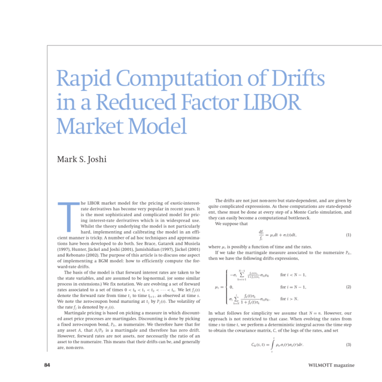
Rapid Computation of Drifts
in a Reduced Factor LIBOR
Market Model
Mark S. Joshi
T
he LIBOR market model for the pricing of exotic-interestrate derivatives has become very popular in recent years. It
is the most sophisticated and complicated model for pricing interest-rate derivatives which is in widespread use.
Whilst the theory underlying the model is not particularly
hard, implementing and calibrating the model in an efficient manner is tricky. A number of ad hoc techniques and approximations have been developed to do both. See Brace, Gatarek and Musiela
(1997), Hunter, Jäckel and Joshi (2001), Jamishidian (1997), Jäckel (2001)
and Rebonato (2002). The purpose of this article is to discuss one aspect
of implementing a BGM model: how to efficiently compute the forward-rate drifts.
The basis of the model is that forward interest rates are taken to be
the state variables, and are assumed to be log-normal. (or some similar
process in extensions.) We fix notation. We are evolving a set of forward
rates associated to a set of times 0 < t0 < t1 < t2 < · · · < tn . We let f j (s)
denote the forward rate from time t j to time tj+1 , as observed at time s.
We note the zero-coupon bond maturing at t j by P j (s). The volatility of
the rate f j is denoted by σ j (s).
Martingale pricing is based on picking a measure in which discounted asset price processes are martingales. Discounting is done by picking
a fixed zero-coupon bond, PN , as numeraire. We therefore have that for
any asset A, that A/PN is a martingale and therefore has zero drift.
However, forward rates are not assets, nor necessarily the ratio of an
asset to the numeraire. This means that their drifts can be, and generally
are, non-zero.
The drifts are not just non-zero but state-dependent, and are given by
quite complicated expresssions. As these computations are state-dependent, these must be done at every step of a Monte Carlo simulation, and
they can easily become a computational bottleneck.
We suppose that
dfi
= µi dt + σi (s)dt,
fi
(1)
where µi is possibly a function of time and the rates.
If we take the martingale measure associated to the numeraire PN ,
then we have the following drifts expressions,

N−1
fk (s)τ k


−σi
σρ

1+fk (s)τ k k ik


k=i+1



µi = 0,




i

fk (t)τk


σk ρik .
 σi
1
+
fk (t)τk
k=N
for i < N − 1,
for i = N − 1,
(2)
for i > N.
In what follows for simplicity we assume that N = n. However, our
approach is not restricted to that case. When evolving the rates from
time s to time t, we perform a deterministic integral across the time step
to obtain the covariance matrix, C, of the logs of the rates, and set
t
Cik (s, t) =
ρir σi (r)σk (r)dr.
(3)
s
84
Wilmott magazine
TECHNICAL ARTICLE 2
This yields an approximation to the total drift across the step
n−1
µi (t − s) ∼ −
k=i+1
fk (s)τk
Cik .
1 + fk (s)τk
If we have precomputed the terms
Note that if i = n − 1, the sum is empty, and we take the value to be zero.
Note that for the calibration of the model, it is only the terms Cik for each
time step that actually matter.
As the terms in this summation depend on i, we need to compute
n − i terms for each value of i, and we need to carry out approximately
n2/2, multiplications. However, for efficiency reduced factor models are
often used in which the matrix C is of rank 2 or 3 instead of n. If we use
the above algorithm we have no gain from this factor reduction, and it
will be the only part of our simulation of order n2 for each step. As a simulation typically has n steps, this means that the drift computation is
growing at rate n3 , and will rapidly become the main drain on computing time. For example if n is 60 then we have of order 216,000 computations for the drifts, versus 3600 for the rest of the simulation.
We show here that the drift computation for one step can be performed using a computation of order nF where F is the number of factors.
The key to our approach is to work with the pseudo-square root of the
covariance matrix rather than the covariance matrix itself.
Thus first we find an n × k matrix A such that
C = AAt .
(5)
(Such a matrix exists if and only if C is of rank k.) As the covariance matrices are fixed this computation need only be carried out once for each
step; in any case the matrix A will be needed for evolving the Brownian
part of the simulation so no additional work is required.
By definition, we have
Cik =
F
Air Atrk .
(6)
r=1
Substituting into (4), we obtain
−
n−1 F
k=i+1 r=1
F
n−1
fk (s)τk
fk (s)τk
Air Atrk = −
Air
Atrk .
1 + fk (s)τk
1
+
f
(s)τ
k
k
r=1
(7)
k=i+1
What does this buy us? The terms in the inner sum do not involve i and
we can therefore reuse them. In particular, if we define
er,i =
n−1
k=i+1
fk (s)τk
At ,
1 + fk (s)τk rk
fi+1 (s)τi+1
1 + fi+1 (s)τi+1
(4)
then all the terms er,i can be computed using only nF multiplications.
We still need to compute
F
Air er,i ,
r=1
for each value of i which results in another nF multiplications. Our computation is therefore of order nF.
In fact, by rethinking our order of computation slightly we can eliminate the second set of multiplications. Given a vector of independent
normals Z = (Z j ), we have to turn them into correlated variates by using
the pseudo-square root. We can therefore absorb the two pseudo-root
multiplications into one and obtain
F
log fi (t) = log fi (s) − 0.5Cii (s, t) +
Air (er,i + Zr ).
(10)
r=1
We have shown that by a judicious reordering, the amount of time spent
on drift calculations can be reduced to a computational time of order nF.
Whilst this idea is not deep it results in considerable time savings when
n is large and F is small, and the approach does not seem to be as well
known as one might expect.
REFERENCES
■ A. Brace, D. Gatarek, M. Musiela, The market model of interest-rate dynamics,
Mathematical Finance 7, 127–155 (1997).
■ D. Brigo, F. Mercurio, Interest Rate Models: Theory and Practice, Springer Finance
2001.
■ C. Hunter, P. Jäckel, M. Joshi, Getting the drift, Risk July 2001.
■ F. Jamishidian, LIBOR and swap market models and measures, Finance and stochastics,
1, 293–330 (1997).
■ P. Jäckel, Monte Carlo Methods in Finance, Wiley 2001.
■ R. Rebonato, The modern pricing of interest rate derivatives, PUP 2002.
BIBLIOGRAPHY
Mark Johsi is Head of Model Evaluation in Royal Bank of Scotland Group Risk
Management. His books “the Concepts of Mathematical Finance” and “C++ Design
Patterns and Derivatives Pricing“ will be published by Cambridge University Press in
Summer 2003.
(8)
we have that
er,i = er,i+1 +
fi+1 (s)τi+1
At
.
1 + fi+1 (s)τi+1 r,i+1
(9)
W
Wilmott magazine
85