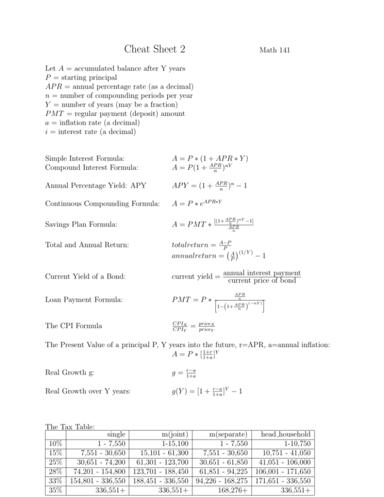
Cheat Sheet 2
Math 141
Let A = accumulated balance after Y years
P = starting principal
AP R = annual percentage rate (as a decimal)
n = number of compounding periods per year
Y = number of years (may be a fraction)
P M T = regular payment (deposit) amount
a = inflation rate (a decimal)
i = interest rate (a decimal)
Simple Interest Formula:
Compound Interest Formula:
A = P ∗ (1 + AP R ∗ Y )
A = P (1 + APn R )nY
Annual Percentage Yield: APY
AP Y = (1 +
Continuous Compounding Formula:
A = P ∗ eAP R∗Y
Savings Plan Formula:
A = P MT ∗
Total and Annual Return:
totalreturn = A−P
P
(1/Y )
−1
annualreturn = PA
Current Yield of a Bond:
current yield =
Loan Payment Formula:
P MT = P ∗
The CPI Formula
CP IX
CP IY
=
AP R n
)
n
−1
R nY
) −1]
[(1+ AP
n
AP R
n
annual interest payment
current price of bond
AP R
n
»
(−nY )
R
1−(1+ AP
n )
–
priceX
priceY
The Present Value of a principal P, Y years into the future, r=APR, a=annual inflation:
1+r Y
A = P ∗ [ 1+a
]
r−a
1+a
Real Growth g:
g=
Real Growth over Y years:
g(Y ) = [1 +
r−a Y
]
1+a
−1
The Tax Table:
single
m(joint)
m(separate)
head household
10%
1 - 7,550
1-15,100
1 - 7,550
1-10,750
15%
7,551 - 30,650
15,101 - 61,300
7,551 - 30,650
10,751 - 41,050
25%
30,651 - 74,200 61,301 - 123,700 30,651 - 61,850 41,051 - 106,000
28% 74,201 - 154,800 123,701 - 188,450 61,851 - 94,225 106,001 - 171,650
33% 154,801 - 336,550 188,451 - 336,550 94,226 - 168,275 171,651 - 336,550
35%
336,551+
336,551+
168,276+
336,551+
n
The mean of x1 , x2 , ...xn is
µ = x1 +x2 +...+x
.
n
2 +(x −µ)2 +...+(x −µ)2
(x
−µ)
n
2
The variance s2 of x1 , x2 , ...xn is
s2 = 1
.
n−1
The standard deviation s is the square root of the variance s2 .
Quartiles of Normal Distributions:
Q1 = mean − .67 ∗ s
Q3 = mean + .67 ∗ s
The 68 − 95 − 99.7 Rule for normal distributions:
68% of the observations fall within 1 standard deviation of the mean.
95% of the observations fall within 2 standard deviations of the mean.
99.7% of the observations fall within 3 standard deviations of the mean.
Given data (x1 , y1 ), (x2 , y2 ), ... (xn , yn ), with means µx , µy and standard deviations sx , sy .
The correlation between variables x and y is
r=
1
(n−1)sx sy
[(x1 − µx )(y1 − µy ) + (x2 − µx )(y2 − µy ) + ... + (xn − µx )(yn − µy )] .
The least squares regression line is
where
y = ax + b.
a = r ∗ ssxy and b = µy − aµx .
For a simple random sample of size n,
count of successes in the sample
the sample proportion of successes is
p0 =
n
The mean of the sampling distribution is pq
p(1−p)
.
and the standard deviation is
n
The 68 − 95 − 99.7 Rule applies here aswell.