Areas
The motivation for our definition of “integral” was the problem of finding the area between
some curve and the x–axis for x running between two specified values. We approximated
the region by a union of thin rectangles and found the exact area by taking the limit as the
width of the approximating rectangles went to zero. We can use exactly the same strategy
to find areas of more complicated regions in the xy–plane. Here are some examples.
Example 1
Find the area of the finite region bounded by y = x2 and y = 6x − 2x2 .
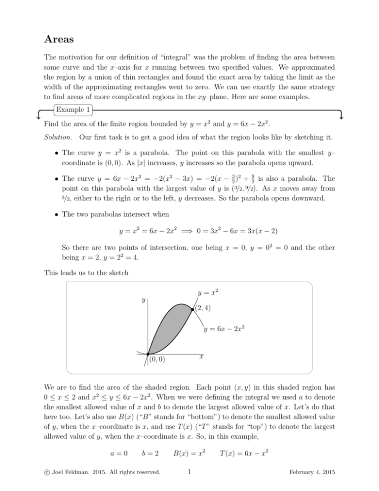
Solution. Our first task is to get a good idea of what the region looks like by sketching it.
• The curve y = x2 is a parabola. The point on this parabola with the smallest y–
coordinate is (0, 0). As |x| increases, y increases so the parabola opens upward.
• The curve y = 6x − 2x2 = −2(x2 − 3x) = −2(x − 23 )2 + 92 is also a parabola. The
point on this parabola with the largest value of y is (3/2, 9/2). As x moves away from
3/2, either to the right or to the left, y decreases. So the parabola opens downward.
• The two parabolas intersect when
y = x2 = 6x − 2x2 =⇒ 0 = 3x2 − 6x = 3x(x − 2)
So there are two points of intersection, one being x = 0, y = 02 = 0 and the other
being x = 2, y = 22 = 4.
This leads us to the sketch
y = x2
y
(2, 4)
y = 6x − 2x2
x
(0, 0)
We are to find the area of the shaded region. Each point (x, y) in this shaded region has
0 ≤ x ≤ 2 and x2 ≤ y ≤ 6x − 2x2 . When we were defining the integral we used a to denote
the smallest allowed value of x and b to denote the largest allowed value of x. Let’s do that
here too. Let’s also use B(x) (“B” stands for “bottom”) to denote the smallest allowed value
of y, when the x–coordinate is x, and use T (x) (“T ” stands for “top”) to denote the largest
allowed value of y, when the x–coordinate is x. So, in this example,
a=0
b=2
c Joel Feldman. 2015. All rights reserved.
B(x) = x2
1
T (x) = 6x − x2
February 4, 2015
and the shaded region is
(x, y) a ≤ x ≤ b, B(x) ≤ y ≤ T (x)
To find the area of this region, we use the same strategy as we used when defining the
integral in §3. of the notes “Definition of the Integral”. We pick a natural number n (that
we will later send to infinity) and subdivide the region into n narrow slices, each of width
. We approximate the area of slice number i by the area of a rectangle. The
∆x = b−a
n
rectangle is the fat dark vertical line in the figure below. On slice number i, the x–coordinate
runs over a very narrow range. (When we were defining the integral we used xi−1 to denote
the smallest x on slice i and we used xi to denote the largest x on slice i.) We pick a number
x∗i , somewhere in that range. We approximate slice i by a rectangle whose bottom is at
y = B(x∗i ) and whose top is at y = T (x∗i ). So we approximate slice number i by a rectangle
• of width ∆x and
• of height T (x∗i ) − B(x∗i ) and so
• of area T (x∗i ) − B(x∗i ) ∆x.
y = B(x) = x2
y
T (x∗i )
y = T (x) = 6x − 2x2
B(x∗i )
a
x∗i
x
b
The desired area is
Z b
n
X
∗
∗
lim
T (xi ) − B(xi ) ∆x =
T (x) − B(x) dx
n→∞
a
i=1
=
Z
2
2
2
(6x − 2x ) − (x ) dx =
0
2
2
x3
x
= 3(2)2 − 23
= 6 −3
2
3 0
Z
2
0
6x − 3x2 dx
=4
Example 1
c Joel Feldman. 2015. All rights reserved.
2
February 4, 2015
Example 2
Find the area of the finite region bounded by y 2 = 2x + 6 and y = x − 1.
Solution. Again we start by sketching the region.
• The curve y 2 = 2x + 6, or equivalently x = 12 y 2 − 3 is a parabola. The point on this
parabola with the smallest x–coordinate is (−3, 0). As |y| increases, x increases so the
parabola opens to the right.
• The curve y = x − 1 is a straight line of slope 1 that passes through x = 1, y = 0.
• The two curves intersect when
x=y+1=
1 2
y − 6 =⇒ 0 = y 2 − 2y − 8 = (y − 4)(y + 2)
2
So there are two points of intersection, one being y = 4, x = 4 + 1 = 5 and the other
being y = −2, x = −2 + 1 = −1.
This leads us to the sketch
y
(5, 4)
(−3, 0)
x
(−1, −2)
y 2 = 2x + 6
y =x−1
We can find the area of this region by approximating it by a union of narrow vertical rectangles, as we did in Example 2. But that’s the hard way. The easy way is to approximate it
by a union of narrow horizontal rectangles. Just for practice, here is the hard solution. The
easy solution is after it.
Hard Solution. We approximate the region by a union of narrow vertical rectangles, each of
width ∆x. Two of those rectangles are illustrated in the sketch
y
(5, 4)
(−3, 0)
x
(−1, −2)
y 2 = 2x + 6
y =x−1
c Joel Feldman. 2015. All rights reserved.
3
February 4, 2015
In this region, x runs from a = −3 to b = 5. The curve at the top of the region is
√
y = T x) = 2x + 6
The curve at the bottom of the region is more complicated. To the left of (−1, −2) the lower
half of the parabola gives the bottom of the region while to the right of (−1, −2) the straight
line gives the bottom of the region. So
( √
− 2x + 6 if − 3 ≤ x ≤ −1
B(x) =
x−1
if − 1 ≤ x ≤ 5
Rb
The area is still given by the formula a T (x) − B(x) dx of Example 2. But to accomodate
our B(x), we have to split up the domain of integration when we evaluate the integral.
Z b
Z −1
Z 5
T (x) − B(x) dx =
T (x) − B(x) dx +
T (x) − B(x) dx
a
−3
−1
Z −1
Z 5
√
√
√
=
2x + 6 − (− 2x + 6) dx +
2x + 6 − (x − 1) dx
−3
−1
Z −1
Z 5
Z 5
√
√
=2
2x + 6 dx +
2x + 6 dx −
(x − 1) dx
−3
−1
−1
We can evaluate the first two integrals by substituting t = 2x + 6, dt = 2 dx, t = 0 when
x = −3, t = 4 when x = −1 and t = 16 when x = 5.
Z 4
Z 16
Z 5
√ dt
√ dt
Area = 2
+
−
(x − 1) dx
t
t
2
2
0
4
−1
3/2 4 3/2 16 2
5
t 1
t 1
x
=2 3
+ 3
−
−x
/2 2 0
/2 2 4
2
−1
h 25
1
i
2
1
= 8 − 0] + [64 − 8] −
−5 −
+1
3
3
2
2
72 24
−
+6
3
2
= 18
=
Easy Solution. The easy way to deal to determine the area of our region is to approximate
by narrow horizontal rectangles, rather than narrow vertical rectangles. Each point (x, y) in
our region has −2 ≤ y ≤ 4 and 21 (y 2 − 6) ≤ x ≤ y + 1. Let’s use
• c to denote the smallest allowed value of y,
• d to denote the largest allowed value of y
• L(y) (“L” stands for “left”) to denote the smallest allowed value of x, when the y–
coordinate is y, and
• R(y) (“R” stands for “right”) to denote the largest allowed value of x, when the y–
coordinate is y.
c Joel Feldman. 2015. All rights reserved.
4
February 4, 2015
So, in this example,
c = −2
1
L(y) = (y 2 − 6)
2
d=4
R(y) = y + 1
and the shaded region is
(x, y) c ≤ y ≤ d, L(y) ≤ x ≤ R(y)
We pick a natural number n (that we will later send to infinity) and subdivide the interval
c ≤ y ≤ d into n narrow subintervals, each of width ∆y = d−c
. We approximate the area of
n
slice number i by the area of a rectangle. The rectangle is the fat dark horizontal line in the
figure below. On slice number i, the y–coordinate runs over a very narrow range. We pick a
number yi∗ , somewhere in that range. We approximate slice i by a rectangle whose left side
is at x = L(yi∗ ) and whose right side is at x = R(yi∗ ). So we approximate slice number i by
a rectangle
• of height ∆y and
• of width R(yi∗) − L(yi∗ ) and so
• of area R(yi∗ ) − L(yi∗ ) ∆y.
y
(5, 4)
y = yi∗
(−3, 0)
L(yi∗ )
R(yi∗ )
x
(−1, −2)
x = L(y) = 21 (y 2 − 6)
x = R(y) = y + 1
The desired area is
lim
n→∞
n
X
i=1
R(yi∗)
−
L(yi∗ )
∆y =
=
Z
d
c
Z
4
−2
R(y) − L(y) dy
− 21 y 2 + y + 4 dy
=
Z
4
−2
(y + 1) −
1
2
y2 − 6
h
i4
= − 16 y 3 + 12 y 2 + 4y
dy
−2
= − 61 (64 + 8) + 21 (16 − 4) + 4(4 + 2)
= −12 + 6 + 24
= 18
Example 2
c Joel Feldman. 2015. All rights reserved.
5
February 4, 2015