ENGR 52 Laboratory 2
Download and expand the week2.zip file, run MATLAB and set the current working directory to the uncompressed week2 folder.
In this section, we’ll look at two different ways of expressing code in an .m file. The first way is as a “script”, in other words, a collection of MATLAB statements that are run whenever we type the name of the file. The second way is a more powerful and refined technique called a “function”, which gives us great flexibility in extending
MATLAB’s capabilities.
1.
Cyl_Volume revisited . We’ll start by looking at the .m file we created last week to solve the cylinder problem. Recall, we were trying to construct a new cylinder tank with a volume 20% greater than the original cylinder, but with the same height. And we were trying to calculate how large the radius should be.
We solved the problem by typing the following statements in the command window: a) r = 8;

the original cylinder radius b) h = 15;

original height c) V = pi*r^2*h  volume of original cylinder d) V = V + 0.2*V

adds 20% to V e) r = sqrt(V/ (pi * h))

new radius
2.
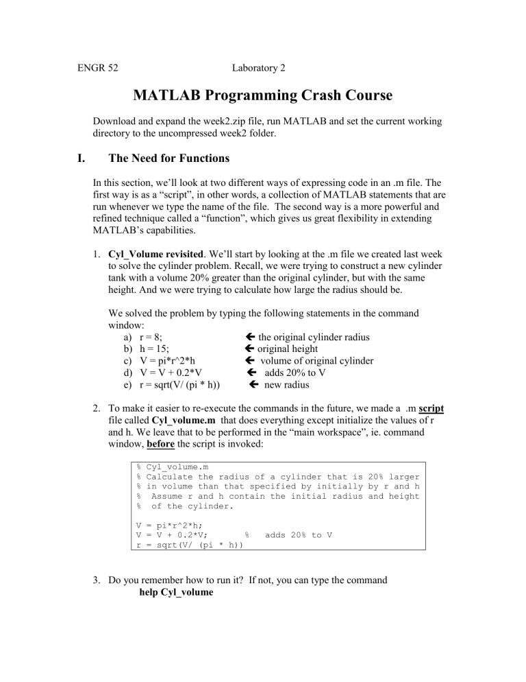
To make it easier to re-execute the commands in the future, we made a .m script file called Cyl_volume.m
that does everything except initialize the values of r and h. We leave that to be performed in the “main workspace”, ie. command window, before the script is invoked:
% Cyl_volume.m
% Calculate the radius of a cylinder that is 20% larger
% in volume than that specified by initially by r and h
% Assume r and h contain the initial radius and height
% of the cylinder.
V = pi*r^2*h;
V = V + 0.2*V; % adds 20% to V r = sqrt(V/ (pi * h))
3.
Do you remember how to run it? If not, you can type the command help Cyl_volume

This will show the contents of the comment lines at the top of the .m file. These hints are telling us that we need to establish initial values for r and h before running the script.
4.
So to do the previous calculation we will now only need to type: a) r = 8; b) h = 15; c) Cyl_volume
5.
If we want to recalculate with different initial parameters, we can just redo the three lines: a) r = 10; b) h = 20; c) Cyl_volume
6.
But this can get tedious. We are shortly going to come up with a new method of performing the calculation where we just have to type:
Cyl_volume(10, 20)

this doesn’t work yet!
This is the same notation used to perform various math calculations such as the cosine of pi cos (pi) or the square-root of 25 sqrt(25);
7.
However, before we move on, let’s take a look at how to clean up the output of this script to make it a little more readable. The following is a look at
Cyl_volume_B.m, which adds some statements (in italics below) to display the results in a nicer format (we have also suppressed normal output on line 11 by adding a ‘;’ at the end)
% Cyl_volume_B.m
% Calculate the radius of a cylinder that is 20% larger
% in volume than that specified by initially by r and h
% Assume r and h contain the initial radius and height
% of the cylinder.
V = pi*r^2*h;
V = V + 0.2*V; % adds 20% to V
%s=sprintf('New Volume = %10.3f',V);
%disp(s) r = sqrt(V/ (pi * h)); s = sprintf('New Radius = %10.3f\n',r); disp(s)
8.
Try this script out now to observe the difference: a) r = 10; b) h = 20; c) Cyl_volume_B

9.
Notice the line: s=sprintf('New Volume = %10.3f',V); This line puts the message and value of V into a “string” variable s, with a certain formatting. Then the disp( ) command displays it. a) In file Cyl_volume_B.m change the floating point format designator
“%10.3f” (meaning the value V is displayed in a width of 10 characters, with 3 after decimal point) to “%8.1f” and observe the difference. b) Add another pair of statements after line 6 to display the old volume in proper formatting. c) However, even with this improvement is still rather tedious to compute the new radius for different values of r and h.
10.
MORE PRACTICE: Write a simple script file Temperature.m that displays a table to convert from degrees Fahrenheit (F) to degrees Celsius (C) over the temperature range 0 to 100 F in increments of 10 degrees. The conversion relation is C = 5*(F-32)/9.
11.
We’re now going to create a function .m file version of Cyl_volume as illustrated in step 6). To begin, close Cyl_volume_B.m
, re-open Cyl_volume.m
and save this file as Cyl_volume2.m. Then add the following line at the very top of the new file: function new_radius = Cyl_volume2( r, h )
This line sets up a function interface : it includes the name of the function
( Cyl_volume2 , which must match the filename) , the parameters it takes (r and h are the placeholders for data in the function call…i.e. the 10 and 20 in
Cyl_volume(10, 20) ) It also indicates that new_radius is the result it will compute and return when it is finished executing. This value then becomes the answer that will show after the function is executed from the command window.
12.
Also change the last line to read: new_radius = sqrt(V/ (pi * h));
This performs the calculation of the value that will be returned from the function: function new_radius = Cyl_volume2( r, h )
% Calculate the new_radius of a cylinder that is 20% larger
% in volume than that specified initially by r and h
V = pi*r^2*h;
V = V + 0.2*V; % adds 20% to V new_radius = sqrt(V/ (pi * h));
13.
Save the file and try out your new function in the command window: a) help Cyl_volume2 b) Cyl_volume2(8, 15) c) Cyl_volume2(10, 20) d) rads = [8:2:16]
Cyl_volume2(rads, 15)

will cause an error

14.
As we’ve already seen, functions can process arrays. The problem with step d) above is certain calculations in our function need to use
.
^ instead of ^ (line 5), and
.
/ instead of / (line 7) to be able to handle cell by cell computations when the parameter r in the function is an array. Make these changes and retry the above example. It should work. This makes it much easier to process cylinders of different radii, because we can now use vectors to list all of the radii we wish to compute.
15.
Try another experiment: a) clear
 clear the workspace b) Cyl_volume2(10, 20) c) check workspace…where are the variables r, h, V, new_radius?
16.
The answer to c) above is that, when we set up the function interface, we essentially isolated what goes on during function execution from the rest of the workspace. In other words, the function performs its calculation on a sort of
“scratch paper” that is discarded as soon as the calculation is completed. This is a good thing, because it prevents us from interfering with variables that may already exist in the main workspace. The variables used inside a function are called “local variables” because they only exist locally when the function is running.
17.
MORE PRACTICE: Make another function Sphere_volume2.m, that solves a similar problem with spheres. The volume of a sphere is 4

r
3
/3, where r is the radius. Given an initial radius, the new function will compute a new radius for a sphere having a volume 30% greater than the initial radius. Hint: use ^(1/3) to take the cube root. Test your function to make sure it works properly.
19.
MORE PRACTICE: Make a function file for a function f1 (filename f1.m), which calculates and returns y = x + 2e
-x
– 3.
function y = f1(x)
y = x + 2*exp(-x) – 3;
18.
MORE PRACTICE: Make a function file to convert a temperature in Fahrenheit to its equivalent Celsius. (filename F2C.m) The conversion is C = 5*(F-32)/9.
The value C should be returned.
Then plot f1(x) over the interval x goes from -1 to 5
20.
Try this demo example to find minimum values of a function of several variables
(A), and Example 3.5-1 (B) Lab 2 Part 1 Demo

Programming is an activity that generally takes a long time for a student to master. In addition, the learning process is fairly dry while things like bugs and program flow issues are overcome. However, we can get a sense of the concepts used in programming (and another cool graphics feature of Matlab) by developing a simple animation. We’ll start with a static plot, then show how to make it come alive.
21.
The initial Brownian.m file just plots a collection of random (x,y) points. It creates 2 vectors, x and y, of 20 points each, where each point is a random number between -0.5 and 0.5. The rand(n, 1) function creates a nx1 vector of uniformly distributed random values between 0 and 1. The variable n is 20 in this case.
The plotting commands create a plot, then fix the axes so they are square.
%Brownian.m
% Display a random scatter plot of points moving under
% Brownian Motion
% part 1--just show the plot of data n = 20; x = rand(n,1) - 0.5; y = rand(n,1) - 0.5; plot(x,y, '.'); axis([-1 1 -1 1]) axis square grid off
22.
The initial Brownian.m file just plots a collection of random (x,y) points. It creates 2 vectors, x and y, of 20 points each, where each point is a random number between -0.5 and 0.5. The rand(n, 1) function creates a nx1 vector of random values between 0 and 1. The variable n is 20 in this case. Try it now!
23.
We can modify the file to make the points move a little bit. First we will need a variable s to control the speed of the particles. Then we will grab a “handle” of our graph in h by saying h = plot(x,y,’.’); having a handle for our graph allows us to change the properties of the points and update them with minimal changes.
Next we will set the EraseMode to allow quicker updates to the plot. Then after a brief 1 second pause, we will adjust the values of x and y slightly using the gaussian randn function, and update their positions (set XData and YData).
%Brownian2.m
% Display a random scatter plot of points moving under
% Brownian Motion
% part 2--added one step change

n = 20; s = .02; Change 1 add line s = .02; x = rand(n,1) - 0.5; y = rand(n,1) - 0.5; h = plot(x,y, '.'); Change 2 add h = axis([-1 1 -1 1]) axis square set(h, 'EraseMode','xor','MarkerSize', 18) Change 3
add to end pause(1) x = x + s*randn(n,1); y = y + s*randn(n,1); set(h, 'XData', x, 'YData', y)
24.
Try this file and notice the small shift the particles make.
25.
Clearly, in order to make this interesting, we’ll need a way to repeat the last group of statements. In other words, we want to continuously add a small random shift to x and y and replot. The following modification sets up a simple “ while loop
” that repeats forever to do this:
%Brownian3.m
% Display a random scatter plot of points moving under
% Brownian Motion
% part 3--full animation n = 20; s = .02; x = rand(n,1) - 0.5; y = rand(n,1) - 0.5; h = plot(x,y, '.'); axis([-1 1 -1 1]) axis square set(h, 'EraseMode','xor','MarkerSize', 18) while 1

Change pause(1) to while 1
drawnow

updates image
x = x + s*randn(n,1);
y = y + s*randn(n,1);
set(h, 'XData', x, 'YData', y) end

ends block of statements to repeat
26.
The statement while 1 means, essentially, while true, or repeat forever. The 1 does not indicate 1 second like in the pause(1) command. Try this script now and you’ll see the particles moving around rapidly. Slow the speed down by changing s to 0.002 or even smaller.

27.
While is not the only loop structure. You can also make a “ for loop
”. Change while 1 to for k = 1:100 and the animation will stop after 100 frames. (Try it!)
Try letting k go to 1000 and notice how much longer it takes. This approach also gives us a variable k that changes (increases by 1) each time the loop executes.
28.
JUST FOR FUN: We can use k in our loop to increase the size of our particles over time. Changing the line set(h, 'XData', x, 'YData') so it reads set(h, 'XData', x, 'YData', y, 'MarkerSize', 18+k/10) will steadily increase the size of the particles until they overlap each other and a strange graphical anomaly occurs.
29.
Another interesting programming structure is the if statement , also known as a branch This statement allows us to execute one or more statements depending on the value of a variable. In this case, since we have a loop variable k, which is changing each time the loop executes, we can insert statements into the loop that change the shape of the marker we are drawing and the marker caller, at certain values of k. Make the change shown in the box below.
…code above… for k = 1:1000
drawnow
x = x + s*randn(n,1);
y = y + s*randn(n,1);
set(h, 'XData', x, 'YData', y,'MarkerSize', 18+ k/10 )
if (k == 300)
 add these
set(h, 'Marker','s','MarkerFaceColor','r') end end
What the change says is “when we get to the 300 th
time through the loop, we will change the marker to a square and the color of the marker to red”. This is done by accessing the image through the plot handle h that we set up before.
30.
We can insert additional branches at other points in the loop execution to change the shape and color again. For example:
…code above… for k = 1:1000
drawnow
x = x + s*randn(n,1);
y = y + s*randn(n,1);
set(h, 'XData', x, 'YData', y,'MarkerSize', 18+ k/10 )
if (k == 300)

set(h, 'Marker','s','MarkerFaceColor','r')
elseif (k == 600)
set(h, 'Marker','d','MarkerFaceColor','g')
end end
31.
See if you can continue this idea and make the marker go back to a blue circle when k reaches 800. The symbol for circle is ‘o’ and the color blue is ‘b’. You can also experiment with marker shapes ‘^’ triangle, ‘V’ triangle, and colors ‘c’ cyan, ‘y’ yellow, ‘k’ black. Also, check out drum.m
another animation in week2.
This section helps you in understanding various relational operators used in both branches and loops. Relational operators compare two values and respond with 1
(true) or 0 (false). For example 3 < 4 evaluates to 1, while 4 ~= 4 evaluates to 0
(false).
32.
Define the variables a = 2, b = 4. Experiment with the following operations and explain what you observe. a) a > b b) a < b c) a >= b d) a <= b e) a == b f) a ~= b
33.
Repeat all the operations above with a = [1 2 3 4] and b = 4. Comment on the results and explain the differences with the above.
34.
Repeat all the operations above with a = [1 3 0 6] and b = [20 1 sin(pi) 9].
Comment on the results and explain the difference with the previous problem.
35.
When comparing vectors, the find function can give a list of cell numbers that satisfy the condition. For example find(a > b) gives the value 2, the only cell where a is bigger than b. Try find on the other five comparisons above (a<b, a == b, etc). Comment on the results.
36.
Once the cell indices are determined using find, you can view them in different ways and set them to other values. a) length(find(a<b))

how many cells meet the condition? b) a(find(a<b))

shows the values of a which are < b c) a(find(a<b)) = 0

changes to 0 values of a which are < b

37.
Problems: Lab 2 Part 3 Problems
38.
Application: Lab 2 Part 4 Problems
39.
The most basic syntax for a branch is the single choice if. Try these out on the command line: a) x = 4; b) if (x < 5)
disp(“good”) end c) change x to 5 and re-run the above (use up arrow to re-enter if statement
40.
There are other forms of the if statement, but it’s easier to test them in a script file. The following file iftest.m is provided to demonstrate the different variations:
% iftest.m test various if statements x=input('enter x: '); disp('1) SINGLE CHOICE TEST') if (x < 5)
disp(' x less than 5') end disp('DUAL CHOICE TEST') if (x < 5)
disp(' x less than 5') else
disp(' x is not less than 5') end disp('3 WAY TEST') if (x < 5)
disp(' x less than 5') elseif (x<10)
disp(' x is between 5 up to but not including 10') else
disp(' x is 10 or more') end disp('4 WAY TEST') if (x < 5)
disp(' x less than 5') elseif (x<10)
disp(' x is between 5 up to but not including 10') elseif (x == 20)
disp ('bingo!') else
disp(' x is 10 or more but not 20') end

41.
MORE PRACTICE: write a matlab script called sin2.m that inputs a scalar x and calculates and displays a value y according to the following rules (use the 3 way test pattern above) y = -x -

for x <=
 y = sin(x) for

<x <=
 y = -x +

for

< x
42.
MORE PRACTICE: write a matlab function called sin3.m that accepts a scalar parameter x and returns a value y according to the same rules as above (use the 3 way test pattern again). Use your function to make a plot showing its behavior over the range -2

<x < 2

43.
MORE PRACTICE: write a matlab script called grade.m that accepts a scalar parameter score and displays the equivalent grade using the standard rules for grading (90 – 100 : A, 80 – 89 : B, etc)
44.
Loops repeat lines of code. The for loop uses a vector to iterate over a pre-defined range of values. Each time through the body of statements is a pass: a) for k = 5:10:35 (that means k = [ 5 15 25 35] ) x = k^2 end
45.
Loops can be nested. We can create a matrix where we count up values in each row. For example, study the code below and run looptest.m to see what it creates.
% looptest.m test of a nested loop.
% this creates a matrix A covering all possible
% permutations of values in the range 0 to 4
A = [0 0 0]; % start with a blank row for c1=0:4
for c2=0:4
for c3=0:4
row=[c1 c2 c3];
A = [A' row']'; % add a new row to A
%(by flipping, adding column, reflipping)
end
end end
A= A(2:end, :) % remove the blank row at the top,
% it's redundant
46.
Problems: Lab 2 Part 5 Problems