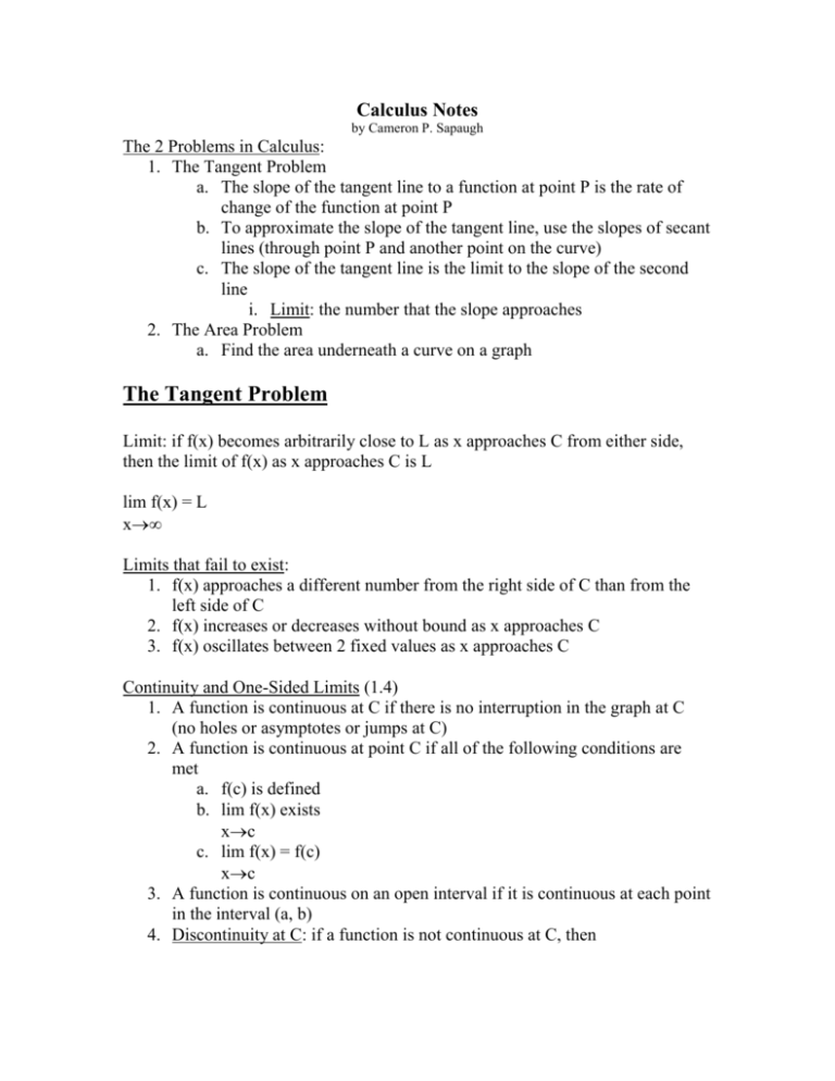
Calculus Notes
by Cameron P. Sapaugh
The 2 Problems in Calculus:
1. The Tangent Problem
a. The slope of the tangent line to a function at point P is the rate of
change of the function at point P
b. To approximate the slope of the tangent line, use the slopes of secant
lines (through point P and another point on the curve)
c. The slope of the tangent line is the limit to the slope of the second
line
i. Limit: the number that the slope approaches
2. The Area Problem
a. Find the area underneath a curve on a graph
The Tangent Problem
Limit: if f(x) becomes arbitrarily close to L as x approaches C from either side,
then the limit of f(x) as x approaches C is L
lim f(x) = L
x
Limits that fail to exist:
1. f(x) approaches a different number from the right side of C than from the
left side of C
2. f(x) increases or decreases without bound as x approaches C
3. f(x) oscillates between 2 fixed values as x approaches C
Continuity and One-Sided Limits (1.4)
1. A function is continuous at C if there is no interruption in the graph at C
(no holes or asymptotes or jumps at C)
2. A function is continuous at point C if all of the following conditions are
met
a. f(c) is defined
b. lim f(x) exists
xc
c. lim f(x) = f(c)
xc
3. A function is continuous on an open interval if it is continuous at each point
in the interval (a, b)
4. Discontinuity at C: if a function is not continuous at C, then
a. removable discontinuity: if the function can be made continuous by
factoring and canceling
b. non-removable discontinuity: cannot be made continuous
5. One-Sided Limits
a. limit from the right
xc+
b. limit from the left
xcRates of Change
1. Position Function: gives height at given point in time
s(t) = ½ gt2 + s0 + s0
g = acceleration due to gravity
v = initial velocity
s = initial height
2. Velocity Function: gives the velocity of an object at time t
s1(t) = v(t)
3. Average velocity on the interval [a, b]
s(b) – s(a)
(b – a)
4. Acceleration Function
s11(t) = a(t)
Derivatives
1. Product Rule
fg1 = f(x)g1(x) + f1(x)g(x)
2. Quotient Rule
fg1 = f1(x)g(x) – f(x)g1(x)
g(x)2
3. Higher Derivatives
a. First f1(x)
b. Second f11(x)
c. Third f111(x)
d. Fourth f4(x)
4. Chain Rule
(d/dx)[f(u)] where u is a function
= f1(u)  u1
5. General Power Rule
(d/dx)[un] = nun – 1  u1
Implicit Differentiation
1. Explicit: y =
2. Implicit: not in y = form
Implicit Differentiation: taking the derivative of y with respect to x. Differentiate
the terms with only x as usual and terms with y require the chain rule using y1 for
the derivative of y
Steps: x2 – 2y3 + 4y = 2
1. Differentiate both sides with respect to x
a. 2x – 6y2  y1 + 4  y1 = 0
2. Collect all y1 terms on the left and all other terms on the right
a. -6y2  y1 + 4y1 = -2x
3. Factor y1 out of the left side
a. y1(-6y2 + 4) = -2x
4. Divide to solve for y1
-2x
a. y1 =
-6y2 + 4
Related Rates
Steps for Solving:
1. Identify all given quantities and qualities to be determined
2. Write an equation involving the variables whose rates of change either are
given or to be determined
3. Implicitly differentiate both sides of the equation with respect to t (time)
4. Substitute all known values into the differentiated equation and solve for
the unknown value
Point Slope Form: (y – y1) = m(x – x1)
Slope Intercept Form: y = mx + b
Slope: m =
y1 – y2
x1 – x2
4 4
1. Parallel Lines: Same Slope (  )
5 5
4 -5
2. Perpendicular Lines: Different Slope (  )
5
4
Graphs and Models
1. Intercepts are points where a graph crosses an axis
a. Find by setting x and y to zero and solving for the other
x-intercept: (#, 0)
y-intercept: (0, #)
Derivatives of Trig Functions
d
1. dx
sinx = cosx
2.
3.
4.
5.
6.
d
dx
d
dx
d
dx
d
dx
d
dx
cosx = -sinx
tanx = sec2x
cotx = -csc2x
secx = secx tanx
cscx = -cscx cotx
Guidelines for Analyzing the Graph of a Function:
1. Find the x- and y-intercepts (set x and y to zero and solve for the other)
2. Find the vertical and horizontal asymptotes
a. Vertical: set denominator equal to zero
b. Horizontal: Lim f(x) = L (divide by highest power on denominator)
x→ ∞
3. Find the relative extrema
a. Find the derivative (f I)and set it equal to zero
b. Find increasing/decreasing intervals (use critical points and vertical
asymptote intervals)
i. Increase to decrease is a relative maximum
ii. Decrease to increase is a relative minimum
4. Find the points of inflection
a. Find the second derivative (f II) and set it equal to zero
b. Find concavity (use critical points and vertical asymptote intervals)
i. Plug the x-value from a change from positive to negative
concavity into the original equation to find your Points of
Inflection
Optimization Problems
1. Identify all quantities and qualities to be determined and make a sketch
2. Write a primary equation for the quantity that is to be maximized or
minimized
3. Write a secondary equation and solve it for one of its variables. Substitute it
into the primary equation
4. Take the derivative and find the critical numbers
a. Critical #’s: set derivative equal to zero
Finding the Point on a Graph Closest to a Certain Point
1. Plug point values into the distance formula
a. d= (x  x )2  (y  y )2
2. Take the derivative inside the square root and set equal to zero
3. Plug that number into the original equation
1
2
1
2

Ex: f(x) = x2 that is closest to the point (2, ½)
1
2
1
2. d= (x  2)2  (x 2  )2
2
 3. d= x 4  4x  17
4
1. d= (x  2)2  (y  )2
1
= 4x3 – 4
 4. f (x)
3

5. 4x – 4 = 0
6. f(1) = (1)2
x=1
closest point = (1,1)
Newton’s Method: the use of a tangent line to approximate the real zeroes of a
function
1. Make an estimate that is close to c (the zero)
a. f(x) = x5 + x – 1
*plug into y1 and use trace x1 = .755
2. Determine a new approximation
a. x 2  x1 
f (x1)
f 1(x1)
b. f1(x) = 5x4 + 1

c. x 2  .755 
*plug into y2 and look at table (using ask)
f (7.55)
f 1 (7.55)
d. x2 = .755 
3. If x2 is within .001 of x1 then you are done. If not, repeat step 2 to find x3,
 x4, x5 … until your within .001.
*the method fails if the function is undefined or the numbers do not
converge
The Area Problem
Antiderivative: if f1(x) is the derivative of f, then f(x) is the antiderivative
f1(x) = 3x2
then…
f(x) = x3
f(x) = x3 + 2
f(x) = x3 – 20
f(x) = x3 + c (c is a constant)
Indefinite Integral: notation for antiderivative
∫ f(x)dx = F(x) + c
Basic Integration Rules:
1. Zero: ∫ 0(dx) = c
2. Constant: ∫ 2(dx) = 2x + c
xn+1
3. Power Rule: ∫ xn(dx) =
+c
n+1
a. add 1 to exponent and then divide by the new exponent
Trig. Integrals
∫ cosx(dx) = sinx + c
∫ sinx(dx) = -cosx + c
∫ sec2x(dx) = tanx + c
∫ secxtanx(dx) = secx + c
∫ csc2x(dx) = -cotx + c
∫ cscxcotx(dx) = -cscx + c
Finding Area
Sigma Notation:
n
 ai  a
1
i 1
 a2  a3 ...  an
i: index of summation (the starting number)
ai: ith term of the sum (function)
n: upperbound (the ending number)
Ex:
4
 2i  2(1)  2(2)  2(3)  2(4)
i 1
Find Area on Calculator
2nd : Stat → Math → Sum → 2nd : Stat → Ops → Seq.
Sum(seq(2x-1,x, a, b))
2x-1: equation
a: lower bound
b: upper bound
Using Sigma Notation to Write the Sum
Ex:
15
5
5
5
5


... 
11 1 2 1 3
1  15
 1 i
5
i1
Summulation Formulas

n
1.
 c  cn
i 1
n(n  1)
2
i 1
n
n(n  1)( 2n  1)
3.  i 2 
6
i 1
n
2.
i 
n
4.
 i3 
i 1
n 2 (n  1) 2
4
Properties of Summation
n
 ka
1.
i
i 1
n
 k  ai
i 1
n
n
n
i 1
i 1
i 1
 (ai  bi )   ai   bi
2.
Lower and Upper Sums to Approximate Area of a Region
n
Lower sum: s(n) :
mi  a  (i 1)(
 f (m )x
ba
)
n
i 1
i
x  width of rectangles
n = # of rectangles
for the interval from [a, b]
n

Upper sum: S(n) :
M i  a  i(
ba
)
n
 f (M )x
i 1
i
Limits of Upper and Lower Sums

lim
lim
s(n) 
S(n)
n 
n 
Area of a Region


Area 
Ci  a  i(
x  (


lim n
 f (Ci )x
n   i1
ba
)
n
ba
)
n
Definite Integrals

b
a
f (x)dx
The integral from a to b of f(x).
a: lower bound

b: upper bound
*Answer is a number
If f is continuous and non-negative on [a,b], then the area of the region bounded
by f, x = a and x = b is

b
f (x)dx
a
Two Special Definite Integrals


a

b

a
f (x)dx  0
f (x)dx    f (x)dx
a
b
a
The Additive Interval Property


b
a
f (x)dx 

c
a
f (x)dx 

b
c
f (x)dx
Properties of Definite Integrals


kf (x)dx  k  f (x)dx
b
b
a
a
 [ f (x)  g(x)]dx  

b
b
a
a
f (x)dx 

b
a
g(x)dx
Limits of Upper and Lower Sums

lim
lim
s ( n) 
S ( n)
x
x
The Area of a Region is Defined as:
lim n
 f (Ci )x
n   i 1
Ci  a  i(
x 
ba
)
n
ba
n
Definite Integrals

b
a
f ( x)dx
a: upper bound
b: lower bound
Two Special Definite Integrals
1.
2.


a
a
a
b
f ( x)dx  0
b
f ( x)dx   f ( x)dx
a
Definite Integral Properties
1.
2.
3.
b
c
b

 kf ( x)dx  k  f ( x)dx
 [ f ( x)  g ( x)]dx   f ( x)dx  
a
b
f ( x)dx   f ( x)dx   f ( x)dx
a
c
b
a
b
a
a
b
b
a
a
g ( x)dx
The Fundamental Theorem of Calculus
If a function f is continuous on [a, b] and F is the antiderivative on f on [a, b],
then:
b

a
f ( x)dx  F (b)  F (a)
The Mean Value Theorem for Integrals
b

a
f ( x)dx  f (c)(b  a)
* f (c )  (
b
1
)  f ( x)dx
ba a
The Second Fundamental Theorem of Calculus
d x
[  f (t )dt ]  f ( x)  F 1 ( x)
dx a
Integration by Substitution (u-substitution)
Indefinite Integrals
 f [ g ( x)]g ( x)dx   f (u)du
1
*u = g(x)
*du=g1(x)dx
Definite Integrals

b
a
f [ g ( x)] g 1 ( x)dx  
g (b)
g (a)
f (u )du
*u = g(x)
*du=g1(x)dx
Integration of Even and Odd Functions
1. If f is an even function (symmetric about the y-axis), then:

a
f (x)dx  2  f (x)dx
a
a
0
2. If f is an odd function (symmetric about the origin), then:

a
a

f (x)dx  0
Numerical Integration: approximating

x 
ba
n
x0  a
x1  x0  x

b
a
f (x)dx
x2  x1  x
xn  b
1. Trapezoidal Rule



b
a

ba
f (x)dx 
[ f (x 0 )  2 f (x1)  2 f (x 2 )... f (x n )]
 2n


2. Simpson’s Rule (if n is even)
ba
[ f (x 0 )  4 f (x1)  2 f (x 2 )  4 f (x 3 )... f (x n )]
3n
Error in Rules: a  x  b
1. Trapezoidal Rule
(b  a) 3
E
max f II (x) 

2 
12n

2. Simpson’s Rule
(b  a) 5
E
max f 4 (x) 
4 
180n



b
a
f (x)dx 
The Natural Logarithmic Function
x1
 ln x  1 dt x  0
t


Logarithmic Properties
If a and b are positive numbers and n is rational:
1. ln(1)  0
2. ln( a  b)  ln( a)  ln( b)


a
3. ln( )  ln( a)  ln( b)
b
4. ln( an )  n  ln( a)
*the number e  2.71828... is the base of the natural log function. ln( e)  1
 Derivatives of Natural Log
 let u be a differential function of x

d
1
1.
ln( x) 
dx
x
d
1 1
2.
ln( u)   u
dx
u

 Ex: Find each derivative





d
1
1
ln( 2x)   2 
dx
2x
x
d
1
2x
2
2.
ln(1 x )
 2x 

2
dx
1 x
1 x 2
d
1
3.
x ln( x)  (1)(ln x)  (x)( )  ln x 1 (Product Rule)
dx
x
d
1
3
4.
(ln x)3  3(ln x)2 ( x )  x (ln x)2 (Chain Rule)
dx
1.