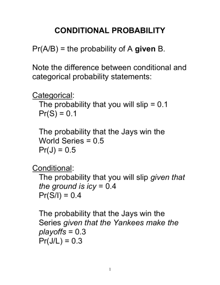
CONDITIONAL PROBABILITY
Pr(A/B) = the probability of A given B.
Note the difference between conditional and
categorical probability statements:
Categorical:
The probability that you will slip = 0.1
Pr(S) = 0.1
The probability that the Jays win the
World Series = 0.5
Pr(J) = 0.5
Conditional:
The probability that you will slip given that
the ground is icy = 0.4
Pr(S/I) = 0.4
The probability that the Jays win the
Series given that the Yankees make the
playoffs = 0.3
Pr(J/L) = 0.3
1
Definition of Conditional Probability
When Pr(B) > 0
Pr(A/B) = Pr(A & B)/Pr(B)
(Remember, you cannot divide by 0.)
Let’s do some examples to convince
ourselves that this is correct.
2
Example 1 (dice):
What is the probability of throwing 3 given
that you throw an odd number?
There are three ways to throw an odd
number: (1, 3, 5).
So, throwing a 3 is one of three possibilities.
Pr(3/odd) = 1/3.
Now let’s use the definition:
Pr(3/odd) = Pr(3 & odd)/Pr(odd)
= Pr(3)/Pr(1, 3, 5)
= (1/6)/(1/2)
= 1/3
3
Example 2 (cards):
What is the probability of drawing a black
card (B) given that you’ve drawn an ace or a
club (A v C)?
There are 13 clubs plus three aces (clubs
include one ace) = 16 cards. 14 of these
are black.
So Pr(B/A v C) = 14/16 = 7/8
Definition:
Pr(B/A v C) = Pr[B & (A v C)]/Pr(A v C)
Pr[B & (A v C)] = Pr(club or ace of spades)
= 14/52
Pr(A v C) = Pr(club or ace of spades or ace
of diamonds or ace of hearts)
= 16/52
Pr(B/A v C) = (14/52)/(16/52)
= 14/16 = 7/8
4
Evidence and Learning from Experience
Imagine that you have the lists of players for
two hockey teams.
Team A: 12 Canadians, 8 other
Team B: 16 Canadians, 4 other
The lists aren’t marked so you choose one
at random and select one player from it.
That player turns out to be Canadian.
What is the probability that you chose from
team B?
We want the probability that the player is
from B given that the player is Canadian,
i.e.:
Pr(B/C) = Pr(B & C)/Pr(C)
5
Pr(C/A) = 0.6
Pr(A) = Pr(B) = 0.5
Pr(C/B) = 0.8
Pr(C/B) = Pr(C & B)/Pr(B)
So:
Pr(C & B) = Pr(B & C) = Pr(C/B)xPr(B)
= 0.8 x 0.5
= 0.4
Similarly,
Pr(A & C) = Pr(C/A)xPr(A)
= 0.3
You can get a Canadian player in one of
two ways: (A & C) or (B & C). These are
mutually exclusive.
So, Pr(C) = Pr(A & C) + Pr(B & C)
= 0.7
Pr(B/C) = 0.4/0.7 = 0.57
Slightly better than 50%.
6
Suppose you pick two players from one of
the lists (alternatively, you pick a second
player from the list you first chose) and both
are Canadian? Now what is the probability
that you chose from B? (You cannot pick
the same name twice.)
Pr(B/C1 & C2) = Pr(B&C1&C2)/Pr(C1&C2)
Pr(B&C1&C2) = Pr(C2/B&C1) x Pr(B&C1)
= 15/19 x 0.4  0.32
Pr(A&C1&C2) = Pr(C2/A&C1) x Pr(A&C1)
= 11/19 x 0.3  0.17
Pr(C1&C2) = Pr(B&C1&C2)+ Pr(A&C1&C2)
 0.49
So:
Pr(B/C1&C2)  0.32/0.49  0.65
7
With the results from two choices we
increase the probability that we chose from
B.
By adding a second result/test we increase
our evidence that we have chosen from B.
We learn by experience by obtaining more
evidence.
Another way of putting it: more evidence of
a given kind increases our certainty in a
conclusion (we knew that anyway but this
shows that conditional probability captures
something correctly).
8
Basic Laws of Probability
Assumptions:
 Rules are for finite groups of
propositions (or events).
 If A and B are propositions (events),
then so are A v B, A & B, ~A.
 Elementary deductive logic (set
theory) is assumed.
 If A and B are logically equivalent
(same events), then Pr(A) = Pr(B).
We’ve already covered the basic laws:
1. Normality: 0  Pr(A)  1
2. Certainty: Pr() = 1
3. Additivity: Pr(A v B) = Pr(A) + Pr(B)
(Where A and B are mutually exclusive)
9
If A and B aren’t mutually exclusive we have
the general disjunction rule:
4. Pr(A v B) = Pr(A) + Pr(B) – Pr(A & B)
Notice we must subtract the “overlap”
between A and B.
This diagram might make it clear:
Pr(A)
Pr(A & ~B)
Pr(A & B)
Pr(B)
Pr(A v B)
Pr(B & ~A)
If we don’t subtract Pr(A & B) we end up
counting it twice. (See the book for an
‘algebraic’ proof.)
10
We also defined conditional probability:
5. Pr(A/B) = Pr(A & B)/Pr(B) (If Pr(B) > 0)
From this it follows that:
6. Pr(A & B) = Pr(A/B) x Pr(B) (If Pr(B) > 0)
This is the general conjunction rule (i.e. it
can be used for events/propositions that are
not independent).
11
Total Probability
Notice that A = (A & B) v (A & ~B)
Why? Remember, every proposition (event)
is true or false (happens or doesn’t). So, if
A is true (happens), then either B is (does)
as well or B is not (does not).
Therefore,
Pr(A) = Pr[(A & B) v (A & ~B)]
= Pr(A & B) + Pr(A & ~B) [why?]
So:
7. Pr (A) = Pr(A/B)Pr(B) + Pr(A/~B)Pr(~B)
(This follows from the definition of
conditional probability.)
12
Logical Consequence
If B logically entails A, then
Pr(B)  Pr(A)
Why? In such cases, B can’t occur without
A occurring so B is equivalent to A & B. As
we just saw:
Pr(A) = Pr(A & B) + Pr(A & ~B),
So, if B entails A, then
Pr(A) = Pr(B) + Pr(A & ~B).
But Pr(A & ~B)  0. Therefore:
Pr(B)  Pr(A) when B entails A.
13
Statistical Independence
If Pr(A) and Pr(B) > 0, then A and B are
statistically independent if and only if:
8. Pr(A/B) = Pr(A)
In other words, B’s truth (occurrence)
doesn’t change the probability of A’s truth
(occurrence).
So, Pr(A & B) = Pr(A) x Pr(B)
Similarly, If A, B and C are independent:
Pr(A & B & C) = Pr(A) x Pr(B) x Pr(C)
And so on.
14
Here an important extension of law 5:
If Pr(E) > 0:
Pr[A/(B&E)] = Pr(A&B&E)/Pr(B&E) (from 5)
i. Pr([A&B]&E) = Pr[(A&B)/E] x Pr(E) (from
5)
ii. Pr(B&E) = Pr(B/E) x Pr(E)
(from 5)
So if we divide i. by ii. we get:
5C. Pr[A/(B&E)] = Pr[(A&B)/E]/Pr(B/E)
This is the conditionalized form of
Pr[A/(B&E)].
15
Odd Question #2:
Remember, A & B entails B (‘A & B’ can’t be
true without ‘B’ being true).
So, it follows that
Pr(A & B)  Pr(B)
16
Bayes’ Rule
H = a hypothesis
E = evidence [Pr(E) > 0]
Pr(H/E) =
Pr(H)Pr(E/H)
Pr(H)Pr(E/H) + Pr(~H)Pr(E/~H)
This is known as Bayes’ Rule.
This follows because H and ~H are mutually
exclusive and exhaustive.
(See chapter 7 in the book for a proof of this
rule).
Try the “Hockey Team” example above
using Bayes’ rule. You’ll see that it works.
17
Sometimes there are more than two
mutually exclusive and jointly exhaustive
hypotheses:
H1, H2, H3, … Hk.
For each i, Pr(Hi)>0.
We can generalize Bayes’ Rule:
Pr(Hj/E) =
Pr(Hj)Pr(E/Hj)
[Pr(Hi)Pr(E/Hi)]
for i = 1, 2, … k.
NOTE: ‘’ just means ‘the sum of’; i.e. you
figure out Pr(H)Pr(E/H) for each hypothesis
and then add them all up.
18
Base rates and reliability
Imagine a test to determine if drinking water
has E. Coli. The test is right 90% of the
time.
Assume 95% of the water in Ontario is free
of E. Coli.
Now you run the test on your drinking water
and it comes up positive for E. Coli. What is
the probability that your water actually has
E. Coli?
Do you think it’s very likely?
After all, the test is very reliable.
19
E = a water sample has E. Coli
~E = a water sample is free of E. Coli
P = the test is positive.
Pr(E) = 0.05 Pr(~E) = 0.95 Pr(P/E) = 0.90
Pr(P/~E) = 0.10 because the test is wrong
10% of the time.
We want to know Pr(E/P). Let’s use Bayes’
Rule:
Pr(E/P) =
Pr(E)Pr(P/E)
P(E)Pr(P/E) + Pr(~E)Pr(P/~E)
= 0.05 x 0.90/[0.05 x 0.90 + 0.95 x 0.10]
= 0.045/0.14
 0.32
So it is only 32% likely that your water is
bad. It is 68% likely that it’s good.
But the test is reliable, so what’s going on
here?
20
Even though the test is very reliable, the
vast majority of water is clean. This is
called the base rate or background
information and it can’t be ignored:
If we tested 1000 samples, only 50 would
have E. Coli, 950 would not (this is the base
rate).
Of the 950 clean samples, the test says:
10% (95) are contaminated;
90% (855) are clean.
Of the 50 contaminated samples, the test
says:
90% (45) are contaminated;
10% (5) are clean.
So, the test would tell us that 140 samples
are contaminated even though only 45 of
those samples are contaminated (5 are
false negatives).
This is why base rates make a difference.
21
Two ideas of reliability:
I. Pr(P/E): how reliable is the test at
identifying contaminated water
given that it is contaminated.
This is a question of how well the
test is designed.
II. Pr(E/P): how trustworthy is the test result
given that it came up positive.
This is a feature of the test plus
the base rate.
We must be careful to take into account
whether a phenomenon is very common or
very rare in the relevant population before
we form a decision about probabilities.
If something is quite rare, even a reliable
test will give more false positives than there
are actual positives.
Hence the test can be reliable (idea I) but
the result unreliable (idea II).
22
Summary
1. 0  Pr(A)  1
2. Pr() = 1
4. Pr(A v B) = Pr(A) + Pr(B) – Pr(A & B)
5. Pr(A/B) = Pr(A & B)/Pr(B)
6. Pr(A & B) = Pr(A/B) x Pr(B)
7. Pr (A) = Pr(A/B)Pr(B) + Pr(A/~B)Pr(~B)
Bayes’ Rule:
Pr(H/E) =
Pr(H)Pr(E/H)
Pr(H)Pr(E/H) + Pr(~H)Pr(E/~H)
23
Homework:
 Do the exercises at the end of chapters 5,
6 and 7
 Go over the “odd questions” in these
chapters until you understand them.
24