AMS312 Spring_2008
Apr 11th
Chapters 6&7 (continued):
Approach 1 – Pivotal Quantity Method
1、 Inference on one population proportion p for large sample test: summary:
Same: H 0 : p  p0
H a : p p0
Same test statistic Z 0 
H 0 : p  p0
H 0 : p  p0
H a : p  p0
H a : p  p0
pˆ  p0
p0 (1  p0 ) / n
 N (0,1) when Ho is true
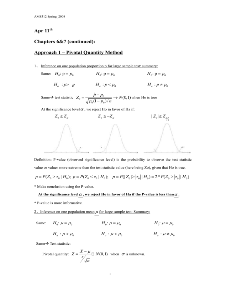
At the significance level  , we reject Ho in favor of Ha if:
Z0  Z
Z 0   Z
| Z0 | Z
2
Definition: P-value (observed significance level) is the probability to observe the test statistic
value or values more extreme than the test statistic value (here being Zo), given that Ho is true.
p  P( Z0  z0 | H 0 ); p  P( Z0  z0 | H 0 ); p  P(| Z0 | z0 | H0 )  2* P(Z0  z0 | H0 )
* Make conclusion using the P-value.
At the significance level  , we reject Ho in favor of Ha if the P-value is less than  .
* P-value is more informative.
2、Inference on one population mean  for large sample test: Summary:
Same:
H 0 :   0
H 0 :   0
H 0 :   0
H a :   0
H a :   0
H a :   0
Same Test statistic:
Pivotal quantity: Z 
X 
s
n
N (0,1) when  is unknown.
1
AMS312 Spring_2008
Z
X 

N (0,1) When  is known.
n
(*Z follows exactly N(0,1) distribution when the population is normal)
Test statistic: Z 0 
X  0
s
n
N (0,1) or Z 0 
X  0

N (0,1)
n
At the significance level  , we reject Ho if:
Z0  Z
Z 0   Z
| Z0 | Z
2
P-values are the same as above (proportion)
Derivation for the 2-sided test:
  P (Type 1 error)=P (reject Ho|Ho)
 P(| Z0 | c | H 0 )  P(Z0  c | H 0 )  P( Z0  c | H 0 )  2P( Z0  c | H 0 )
Hence P( Z 0  c | H 0 )  
2
Therefore, we reject Ho at  if: | Z 0 | Z
2
Example 1 (Problem 6.2.10 from Page439)
At a class research project, Rosaura wants to see whether the stress of final exams elevates the
blood pressures of freshmen women. When they are not under any untoward duress, healthy
18-year-old women have systolic blood pressures that average 120mmHg. If Rosaura finds that
the average blood pressure for the 50 women in statistics 101 on the day of the final exam is 125.2
with sample standard deviation 13 mm Hg, what should she conclude? Set up and test an
appropriate hypothesis.
Solution: This is test on one population mean for large sample.
N=50, X  125.2 , 0  120 s  13   0.05
H 0 :   120 v.s. H a :   120
Z0 
125.2  120
132
 2.8
50
Since Zo=2.8>1.645, we reject Ho at   0.05
P-value=0.0026, since P-value<0.05, we reject Ho
If   0.01 : since now P-value is still smaller than 0.01, we reject Ho.
2
AMS312 Spring_2008
3、Inference on one population mean  , small sample test, normal population:
Same:
H 0 :   0
H 0 :   0
H 0 :   0
H a :   0
H a :   0
H a :   0
Now the pivotal quantity is:
T
X 
s
n
tn 1 Exactly
William S. Gosset (1876 -1937), inventor of the Student’s t-distribution.
Example 2 (Page 490): Pica is a children’s disorder characterized by a craving for
nonfood substances such as clay, plaster, and paint. Anyone affected runs the risk of
ingesting high levels of lead, which can result in kidney damage and neurological
dysfunction. Checking a child’s blood lead level is a standard procedure for
diagnosing the condition.
Among children between the ages of six months and five years, blood lead levels of
16.0mg/l are considered “normal”. Recently, a random sample of twelve children
enrolled in Molly’s Mighty Bear Nursery had their blood lead levels checked. The
resulting sample mean and sample standard derivation were 18.65 and 5.049,
respectively. Can it be concluded that children at this particular facility tend to have
higher lead levels? At the   0.05 level, is the increase from 16.0 to 18.65 statistically
3
AMS312 Spring_2008
significant?
Solution:
H 0 :   16
H a :   16
Average lead level for all children in Milly’s daycare
X  1 8 . 6, 5s=5.049 ( s 
(X
i
 X )2
n 1
)   0.05
Assuming the blood lead distribution for the population is normal
Test statistic: T0 
X  0 18.65  16.0

 1.82
s
5.049
n
12
At   0.05 , we will reject the null hypothesis if T0  tn 1,  t11,0.05  1.7959
Now 1.82>1.7959 hence we reject the null hypothesis.
Approach 2 -- Likelihood ratio test (LRT):
H0 : 
Ha : c
Data: X1 , X 2 ,..., X n : i.i.d. follow p.d.f. f (x;  )
Let     c
n
Likelihood function: L   f ( xi ; )
i 1

max  L
1
max  L
If Ho is true, then  1 so we should reject Ho if   c  1
Use the definition of Type I error rate (significance level) to derive the
threshold value c as usual. That is: Set P(  c | H 0 )   and then solve for c
Example 3: Let X 1 , X 2 ,..., X n
N (  ,  2 ) ,  2 is unknown. Please derive the LRT
for  .
H 0 :   0   {( 0 ,  2 ),  2 positive}
H a :   0   {(  ,  2 ),   0 &  2 positive}
4
AMS312 Spring_2008
    c  {( ,  2 ),   R,  2 positive}
n
n
L   f ( xi ;  ,  )  
i 1

2
i 1
max   
0 ,
2
0
L

1
2
2
( X i   )2
e
2 2

n
2
 (2 ) e
2

 ( X i   )2
2 2
MLE’s for  and  2 in 
max R , 2 0 L
For the numerator:
n
( X   )2
n
n
max    , 2 0 ln L0  max    , 2 0 [ ln(2 )  ln( 2 )   i 2 0 ] (*)
0
0
2
2

i 1
Then
d (*)
n 1  ( X i  0 )


 0  ˆ 02 
2
2
4
d
2
2
Hence max  L  (2ˆ )e
2
0

n
2
[
(X
i
 0 ) 2
n
2  ( X i  0 ) 2
n

n
] 2e

n
2
Similarly, we can derive:
For the denominator:
max R , 2 0 L  ˆ  X ,  2 
(X
i
 X )2
n
2  (X i  X 2)
m a xL  (
2 e )
[
n

2
Therefore,   [
n
2
(X   )
(X  X )
i
0
2

]
2

n

2
e]
n
2
n
2
i
At the significance level  , we reject the null hypothesis if   c  1
c is the value such that:
P(  c | H0 ) 
(X   ) ]  c | H :    )  
(X  X )
(X   )  c | H :    )  
 P(
(X  X )
2
 P([
i
0

n
2
0
2
0
i
2
i
0
*
2
0
0
i
5
AMS312 Spring_2008
And,
n
n
n
n
i 1
i 1
i 1
i 1
 ( X i   0 ) 2   ( X i  X ) 2   ( X   0 ) 2   ( X i  X ) 2  n( X   0 ) 2
(X
(X
n
i 1
i
 0 ) 2
 1
2
i  X)
n( X  0 ) 2
n
(X
i 1
i
 1
 X )2
( X  0 ) 2
n
n
 1
(t0 ) 2
n
n 1
n 1
 ( X i  X )2
i 1
n 1
Hence the above formula becomes:
P((t0 )2  c** | H 0 :   0 )  
 P(T0  c** | H 0 )  P(T0   c** | H 0 )  
Given H 0 : T0
Symmetric, therefore we reject Ho at significance level  if:
(T0 )2  (tn 1, )2 | T0 | tn 1,
2
6
2
tn1