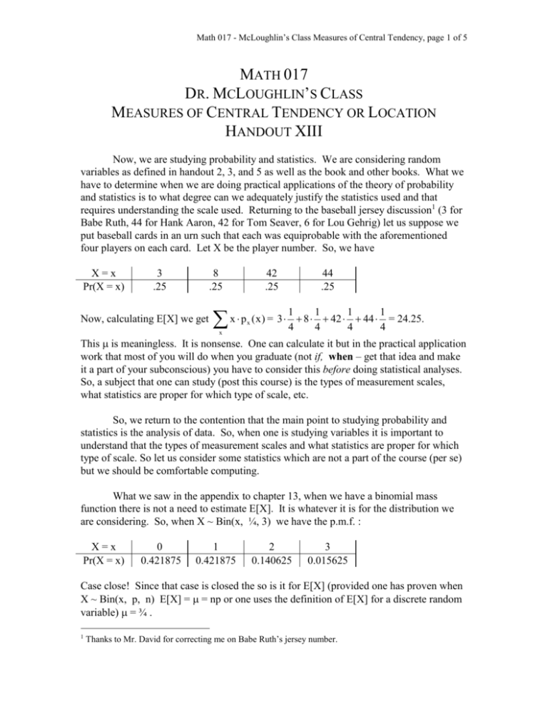
Math 017 - McLoughlin’s Class Measures of Central Tendency, page 1 of 5
MATH 017
DR. MCLOUGHLIN’S CLASS
MEASURES OF CENTRAL TENDENCY OR LOCATION
HANDOUT XIII
Now, we are studying probability and statistics. We are considering random
variables as defined in handout 2, 3, and 5 as well as the book and other books. What we
have to determine when we are doing practical applications of the theory of probability
and statistics is to what degree can we adequately justify the statistics used and that
requires understanding the scale used. Returning to the baseball jersey discussion1 (3 for
Babe Ruth, 44 for Hank Aaron, 42 for Tom Seaver, 6 for Lou Gehrig) let us suppose we
put baseball cards in an urn such that each was equiprobable with the aforementioned
four players on each card. Let X be the player number. So, we have
X=x
Pr(X = x)
3
.25
8
.25
Now, calculating E[X] we get
42
.25
44
.25
 x  p (x) = 3  4  8  4  42  4  44  4 = 24.25.
1
1
1
1
x
x
This  is meaningless. It is nonsense. One can calculate it but in the practical application
work that most of you will do when you graduate (not if, when – get that idea and make
it a part of your subconscious) you have to consider this before doing statistical analyses.
So, a subject that one can study (post this course) is the types of measurement scales,
what statistics are proper for which type of scale, etc.
So, we return to the contention that the main point to studying probability and
statistics is the analysis of data. So, when one is studying variables it is important to
understand that the types of measurement scales and what statistics are proper for which
type of scale. So let us consider some statistics which are not a part of the course (per se)
but we should be comfortable computing.
What we saw in the appendix to chapter 13, when we have a binomial mass
function there is not a need to estimate E[X]. It is whatever it is for the distribution we
are considering. So, when X ~ Bin(x, ¼, 3) we have the p.m.f. :
X=x
Pr(X = x)
0
0.421875
1
0.421875
2
0.140625
3
0.015625
Case close! Since that case is closed the so is it for E[X] (provided one has proven when
X ~ Bin(x, p, n) E[X] =  = np or one uses the definition of E[X] for a discrete random
variable)  = ¾ .
1
Thanks to Mr. David for correcting me on Babe Ruth’s jersey number.
Math 017 - McLoughlin’s Class Measures of Central Tendency, page 2 of 5
Recall:
If X is a discrete random variable and the function given by f(x) = Pr(X = x) for each x in
the domain of the function is the p. m. f. at x, then the expected value (or mean) of X is
E[X] =
 x  f ( x) .
x
There are estimators for  and there are other measures of central tendency.
Definition 1: Let X be a random variable. The mode of X is the value of X, say x0, where
the p.d.f. or p.m.f. is the maximum value. Denote the mode as mo.
Definition 2: Let X be a random variable. The median of X is the value of X, say x1,
where the Pr(X  x1) = Pr(X  x1). Denote the median as md.
Definition 3: Let X be a random variable with a probability mass or density function. Let
X1, X2, X3, . . . , Xn be a finite random sample for X. The arithmetic mean of the
1
sample is the value X where X =
n
n
X .
j
j1
Definition 4: Let X be a random variable with a probability mass or density function. Let
X1, X2, X3, . . . , Xn be a finite random sample for X. Let w1, w2, w3, . . . , wn be real
numbers signifying the ‘importance’ of X1, X2, X3, . . . , Xn respectively. The weighted
n
 (w  X )
j
arithmetic mean of the sample is the value WX where WX =
j
j1
.
n
w
j
j1
Definition 5: Let X be a random variable with a probability mass or density function. Let
X1, X2, X3, . . . , Xn be a finite random sample for X. The mode of the sample is the
value of X which occurs most frequently such that there is at least one value that occurs
with lesser frequency.
Definition 6: Let X be a random variable with a probability mass or density function. Let
X1, X2, X3, . . . , Xn be a finite random sample for X. The median of the sample is the
value of X which occurs in the centre of ordered values of the sample if there are an odd
number of values and it is the arithmetic mean of the centre two values if there are an
even number of values.
Definition 7: Let X be a random variable with a probability mass or density function
where X > 0 for all X where X > 0 for all X. Let X1, X2, X3, . . . , Xn be a finite random
n
sample for X. The geometric mean of the sample is the value G where G = n
X
j1
j
.
Math 017 - McLoughlin’s Class Measures of Central Tendency, page 3 of 5
Definition 8: Let X be a random variable with a probability mass or density function. Let
X1, X2, X3, . . . , Xn be a finite random sample for X where X  0 for all X.. The
n
harmonic mean of the sample is the value H where H = n
.
1
Xj
j1

There are others kinds of means used in different applied areas:
Definition 9: Let X be a random variable with a probability mass or density function. Let
X1, X2, X3, . . . , Xn be a finite random sample for X where X > 0 for all X. The
quadratic mean of the sample (or the root mean squared) is the value R where
R=
1
n
n
 (X ) .
2
j
j1
Definition 10: Let X be a random variable with a probability mass or density function.
Let X1, X2, X3, . . . , Xn be a finite random sample for X where X > 0 for all X.
The p-power mean of the sample (there are many for different values of p
1
(or the Hölder mean)) is the value P where P =
n
p
n
 (X ) .
p
j
j1
Notice for p = 2 it is the root mean squared.
Notice for p = 1 it is the arithmetic mean.
Notice for p = 0 it is the geometric mean.
Notice for p = -1 it is the harmonic mean.
Definition 11: Let X be a random variable with a probability mass or density function
where X > 0 for all X. Let X1, X2 be a random sample (X1  X2) of size 2 for X where X
> 0 for all X. The Heronian mean of the sample is the value HE where
1
HE = (X1  X1  X 2  X 3 ) .
3
Math 017 - McLoughlin’s Class Measures of Central Tendency, page 4 of 5
Definition 12: Let X be a random variable with a probability mass or density function
where X > 0 for all X. Let X1, X2 be a random sample (X1  X2) of size 2 for X where X
> 0 for all X. The logarithmic mean of the sample is the value L where
X  X2
X1  X 2
L=
= 1
.
X1
ln(X1 )  ln(X 2 )
ln( )
X2
Definition 13: Let X be a random variable with a probability mass or density function
where X > 0 for all X. Let X1, X2 be a random sample (X1  X2) of size 2 for X where X
> 0 for all X. The identric mean of the sample is the value I where
1
1  (X1 ) X1  X1  X2
I = 

e  (X 2 ) X2 
Definition 14: Let X be a random variable with a probability mass or density function
where X > 0 for all X. Let X1, X2, X3, . . . , Xn be a random sample (all distinct) for X
where X > 0 for all X. Seppo Mustonen of the Department of Statistics at the University
of Helsinki defines the logarithmic mean of the sample is the value L where
n
L = (n – 1)!

i 1









n

j1
j i



Xi

.
X i 
ln( )
Xj 


PHEW! Ridiculous. Needless to say, there are many estimators.
Math 017 - McLoughlin’s Class Measures of Central Tendency, page 5 of 5
Computational Examples:
Suppose the X i are given by X1 = 0.1, X2 = 0.1, X3 = 0.1, and X4 = 10.
X = 2.575, G =
4
40
1
, G  0.316227766, H =
, H  0.13, mo = 0.1, md = 0.1, etc.
301
100
Suppose the X i are given by X1 = 0.1, X2 = 10, X3 = 10, and X4 = 10.
X = 7.525, G = 4 100 , G  3.16227766, H =
40
, H  0.39 mo = 10, md = 10, etc.
103
Suppose the X i are given by X1 = 1, X2 = 2, X3 = 3, and X4 = 4.
X = 2.5, G =
4
24 , G  2.2133638394, H = 0.48, m0 does not exist, md = 2.5, etc.
The geometric, logarithmic, and harmonic means are used by Chemists and
Chemical Engineers. The geometric mean is used when averaging numbers that involve
growth data. The mean relative volatility between two components in a distillation
column is based on the geometric mean. The logarithmic mean is used in the heat
transfer to determine the mean temperature difference between hot and cold streams
flowing in a heat exchanger. The harmonic mean is the reciprocal of the arithmetic mean
of the reciprocals. It is used, for example, to calculate the mean overall heat transfer
coefficient, Vo, in a heat exchanger.
“Many wastewater dischargers, as well as regulators who monitor swimming beaches and
shellfish areas, must test for and report fecal coliform bacteria concentrations. Often, the data must be
summarized as a "geometric mean" (a type of average) of all the test results obtained during a
reporting period. Typically, public health regulations identify a precise geometric mean concentration
at which shellfish beds or swimming beaches must be closed.
A geometric mean, unlike an arithmetic mean, tends to dampen the effect of very high or low
values, which might bias the mean if a straight average (arithmetic mean) were calculated. This is
helpful when analyzing bacteria concentrations, because levels may vary anywhere from 10 to 10,000
fold over a given period.” - Dr. Joe Costa, Buzzards Bay Project
I notice on the State Department web-site there was a tutorial on bio-terrorism
which mentions the geometric mean.
The Heronian arises in the determination of the volume of a pyramidal frustum.
For further investigation:
Bullen, P. S.; Mitrinovic, D. S.; and Vasic, P. M. (1988). Means and Their Inequalities.
Dordrecht, Netherlands: Reidel.
Last revised 2 Oct. 2006
© 2003 – 2006 M. P. M. M. M.