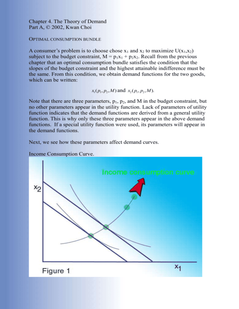
Chapter 4. The Theory of Demand
Part A, © 2002, Kwan Choi
OPTIMAL CONSUMPTION BUNDLE
A consumer’s problem is to choose chose x1 and x2 to maximize U(x1,x2)
subject to the budget constraint, M = p1x1 + p2x2. Recall from the previous
chapter that an optimal consumption bundle satisfies the condition that the
slopes of the budget constraint and the highest attainable indifference must be
the same. From this condition, we obtain demand functions for the two goods,
which can be written:
x1 ( p1 , p2 , M ) and x2 ( p1 , p2 , M ).
Note that there are three parameters, p1, p2, and M in the budget constraint, but
no other parameters appear in the utility function. Lack of parameters of utility
function indicates that the demand functions are derived from a general utility
function. This is why only these three parameters appear in the above demand
functions. If a special utility function were used, its parameters will appear in
the demand functions.
Next, we see how these parameters affect demand curves.
Income Consumption Curve.
An Engel Curve shows the relationship between demand and income.
A good is normal if an increase in income raises its consumption.
A good is inferior if an increase in income lowers its consumption.
Income elasticity of demand for x
M 
%x
x / x
x M


.
%M M / M M x
Normal goods: income elasticities are positive.
Inferior goods: income elasticities are negative.
2
Normal good: As M increases, X increases.
Inferior good: Not all goods can be inferior goods.
3
Price consumption Curve and Demand Curve
4
Income and Substitution Effects
Hicksian Decomposition
Initial equilibrium is at point a. Suppose the price of good 1 declines, which
causes a counterclockwise rotation of the budget line.
The substitution effect measures the change in consumption, holding utility
constant, in response to a change in the relative price, p1 / p2 . This is measured
by Arrow #1 in Figure 5.
Because of this decline in the relative price, it does not cost as much to
maintain the same level utility as before. Since the actual money income M has
not changed, this price decline results in an increase in a sort of “real income.”
The fictitious budget line at point b, is parallel to the new budget line. The gap
between the two budget line shows the increment of real income. Given this
increment, the consumer moves from point b to c. This movement is the income
effect. The total effect is the sum of the two effects.
5
Slutsky Decomposition of the price change.
Δx1/Δp1 = Δx1/Δp1│u - x1(Δx1/ΔM)
In the case of an inferior good, the increment in “real income” causes a decline
in consumption. In a rare case, this negative income effect can more than offset
the initial substitution effect. Figure 6 illustrates such a case where
consumption of the good actually declines (point c is to the left of point a) in
response to a decline in its price.
6
Compensated and Marshallian (uncompensated) demand curves
Marshallian demand: M is fixed
Compensated demand: U is fixed.
In Figure 7a, Marshallian demand curve is denoted by DM and the compensated
demand curve by Dc. The substitution effect is always negative. Thus, the
compensated demand curve is always negatively sloped. Marshallian demand
curve is not always negatively sloped. If the demand curve for a good is
positively sloped, we call it a Giffen good. Thus, we can say that the
Marshallian demand curve is negatively sloped, except for the Giffen good.
However, Giffen good is rarely observed. There was a great famine in Ireland
during the 19th century. Their staple diet consisted mainly of potato and meat.
During the famine, the price of potato increased and the Irish farmers consumed
more potatoes. We assume that demand curve is negatively sloped from now on.
In the case of a normal good, Marshallian demand curve is always flatter than
the compensated demand curve. For an inferior good, the reverse relationship is
true.
7
COST OF LIVING ADJUSTMENT
Prices change over time. Sometimes a manager or a vice president of a
multinational company assigned to move to a foreign city receives a long term
contract which includes a cost of living adjustment based on the consumer price
index (CPI).
Managers of multinational firms are often reluctant to move to foreign cities. In
addition to coping with a different culture, they are facing different prices in
another city or country. The idea is to allow managers to maintain their lifestyle
and induce them to accept assignments in foreign cities. It is necessary then to
adjust their income so that with the new income the manager is able to afford
the previous consumption bundle at the time the contract is made.
Price decline
The initial equilibrium is at point a. If the price of good 1 declines, a cost of
living adjustment requires a pay cut, after which the consumer is still able to
purchase the original consumption bundle a. But once the compensation is
8
made, he has no obligation to stay at the initial equilibrium. He does not stay
there, but moves to point b, which is on a higher indifference curve U '.
Price increase
The initial equibrium  a. An increase in the price of good 1 rotates the budget
line from 1 to 2. In this case, budget line 2’ is requires to purchase the original
consumption bundle a. This difference between the two budget lines (2’ – 2) is
the cost of living adjustment. But will the consumer stay at point a? No. he
moves to a better point, b.
These two diagrams demonstrate that cost of living adjustment
overcompensates the consumer, and makes him better off.
Price Decline  Income may be cut for the cost of living adjustment.
Price Increase  Income must be increased for the cost of living adjustment.
9
MARKET DEMAND CURVE
Market Demand: a horizontal summation of individual demand curves.
Normally, a business firm does not care whether more demand comes from
James Bond or from Lady Bush. The firms are concerned with the market
demand curve.
Market demand is also negatively sloped, since the individual demand curves
are negatively sloped. At lower prices consumers demand more.
Now let us turn our attention to the sensitivity of the relationship. Price
sensitivity of demand may be greater for some goods than for others. Even for
the same product, sensitivity changes along the demand curve.
Q
%Q
Q P
Q



.
P
%P
Q P
P
ΔQ cannot be compared among different demands. For example, as price
declines by $1, ΔQ = 2 for automobiles, but ΔQ = 3 bushels for corn. We
cannot say that ΔQ = 2 cars is bigger than ΔQ = 3 bushels. To compare
sensitivity of changes in demand, we need a relative concept.
PED relates to percentage change in quantity demanded to percentage change
in price. It is a unit free measure, and it can be compared across commodities.
For this reasons, we can compare the elasticities of demand for automobiles in
Germany and in Japan, although their demand curves are expressed in terms of
mark and yen prices.
10
MEASUREMENT OF PED
Point elasticity (Є)  use initial price and quantity
P (price)
Q (quantity)
20
100
10
200
200  100
Є  =  100  2.
10  20
20
Next,
100  200
1
Є  =  200  .
20  10
2
10
Thus, PED can change dramatically, depending on what point is used as the
basis. This example shows that point elasticity is reliable only for small price
changes, but not for large price changes. To avoid this problem, we sometimes
use arc elasticity, which is measured in a price interval.
Arc elasticity  use average price and average quantity.

Q /(Q1  Q2 )
.
P /( P1  P2 )
Using, the above example, we have
Є =
100 /150
 1.
10 /15
This means that revenue remains unchanged by price changes.
11
DEMAND FOR MODEL T
In 1905, the average automobile produced in the US cost more than the
average Japanese car in 1980. Many automobile firms hired skilled mechanics
and produced handcrafted automobiles. However, simplicity and automation
were the key to the automobile industry’s future. Henry Ford introduced
assembly line to automobile production. He introduced model T in 1909. The
following table shows the success of Model T. (Source lost)
Fill out the blanks:
Year
Price
Q demanded
1909
$900
58,000 cars
1914
$440
472,000
1916
$360
730,000
ε
ε
arc ε
***
***
***
The record sale between 1910 and 1920 confirmed the wisdom of Chinese
saying (Low margin sells volumes) That is, it is better to sell many cars at a
small margin than to sell few cars at a high margin.
This statement is true only if demand is sufficiently elastic.
Elasticity Categories:
Є = .5 means that as price declines by 1%, quantity demanded increases
by 0.5%.
Actual Quantity changed
Q = Є P.
Special Cases:
Є > 1  demand is price elastic.
Є < 1  demand is price inelastic.
Є = 1  demand is unitary price elastic. (In this case, the demand curve is a
rectangular hyperbola. The area of the square generated by any point on the
demand curve is the same.)
Є =  demand is perfectly elastic, horizontal demand curve.
Є = 0  demand is perfectly inelastic, a vertical demand curve.
12
13
Graphical Measurement of Point Elasticity of Demand
To measure the price elasticity of demand at a given point C on the demand
curve, draw a tangent line AB at point C.
ΔQ = AQ*, ΔP = OP*.
ΔQ/ΔP = AQ*/OP*.
P/Q = OP*/OQ*
Then Є = AQ*/OQ* = AC/BC
14
Linear Demand and PED
A point on a linear demand curve bisects it. When the top and the bottom
segments are of equal length, (e.g., AC = CE), PED = 1. As one moves upward
from that point on the demand curve, the bottom segment becomes longer than
the top, and hence PED increases, approaching  at point A. On the other hand,
a downward movement along the demand curve reduces the bottom segment,
approaching zero at point E. (The book expresses elasticities as negative
numbers.)
15
TOTAL REVENUE AND ELASTICITY
There is a straightforward relationship between TR and PED. TR is defined by
PQ, and is described by the rectangular area generated by a point on a given
demand curve.
Useful Formula:
Let Z = XY, and let Xˆ  X / X denote a percentage change in X.
Next, Z changes to Z '. Then
ˆ ˆ ) XY .
Z '  (1  Xˆ ) X (1  Yˆ )Y  (1  Xˆ  Yˆ  XY
ˆ ˆ.
Thus, Zˆ  Xˆ  Yˆ  XY
ˆ ˆ is even smaller. For
If the percentage changes X̂ and Yˆ are small, then XY
ˆ ˆ  0.0006. Thus, for small percentage
instance: if Xˆ  0.02 and Yˆ = 0.03, then XY
ˆ ˆ. Then we have the following formulas,
changes, it is safe to ignore the term, XY
which are useful for ready estimation.
If Z = XY, then Zˆ  Xˆ  Yˆ.
If Z = 1/X, then Zˆ   Xˆ .
If Z = X/Y, then Zˆ  Xˆ  Yˆ.
Using these formulas, we have
 Qˆ 
Rˆ  Pˆ  Qˆ  Pˆ 1    Pˆ (1   ).
ˆ
 P
(1) Inelastic Demand (є < 1)  P̂ and R̂ have the same sign. That is, price and
revenue move in the same direction.
Example: є = 0.5, and P̂ = - 10%. Then Rˆ  10%(1  0.5)  5%.
(2) Elastic Demand (є > 1)  P̂ and R̂ have the opposite signs. Price and
revenue move in the opposite direction.
Example: є = 2 P̂ = - 10%. Then Rˆ  10%(1  2)  10%.
(3) Unitary Elastic Demand (є = 1).
16
R̂ = 0. That is, revenue is unaffected by price change.
Gains and losses from a price decline
In Figure 10, at point A, demand is infinitely elastic. Thus, a price decline will
increase revenue.
At point B, PED is 3, and demand is elastic. A price decline still increases
revenue.
At point C, demand is unitary elastic. At this point revenue is maximized.
At point D, demand is inelastic, and a price decline reduces revenue.
At point E, demand is perfectly inelastic. Hence, a price increase will increase
revenue.
Mar-5-09 11:26am/5/2009 17:26 GMT
From: www.businessweek.com
OVER A BUCK FOR DINNER? OUTRAGEOUS
Gary M. Rodkin found out the hard way the perils of pushing up the price of a Banquet frozen
dinner. When the chief executive of ConAgra Foods tried to recoup high commodity costs by
hiking the list price of Banquet products in September, many retailers began charging up to
$1.25 a meal. The response from shoppers used to paying $1? The cold shoulder.
A chastened Rodkin soon discovered why Banquet had become an $800 million brand for the
$12 billion-a-year Omaha food company. "The key component for Banquet dinners--the key
attribute--is you've got to be at $1," he says. "Everything else pales in comparison to that."
The resulting sales drop forced ConAgra to peddle excess dinners to discounters and
contributed to a 40% drop in its stock price in 2008. It also prompted Rodkin, 56, to move
ConAgra further into austerity mode. He expects to cut $250 million in costs this fiscal year,
which ends in May, and trim close to the same amount next year. Some of the savings will
come from moves such as centralizing purchasing and shipping. But Rodkin is also pushing
for creative ways to hold down costs in ConAgra's 37 brands, which include Chef Boyardee,
Marie Callender's, Hunt's, and Healthy Choice.
Rodkin's first priority: bringing the cost of Banquet dinners back to a buck. ConAgra first
tossed out pricey items such as barbecued chicken and country-fried pork in favor of grilled
meat patties and rice and beans. It also shrank portion sizes while swapping in cheaper
ingredients, such as mashed potatoes for brownies. What Rodkin didn't sacrifice was variety,
with close to 100 Banquet-branded products.
ConAgra has made other moves on the cheap. It's reducing the number of can sizes in lines
such as Hunt's and Van Camp's to save on manufacturing costs. The company is cutting
investment in mature brands such as Egg Beaters and Hebrew National to free up money for
growing lines such as Orville Redenbacher's popcorn. It has innovated at low cost by adapting
the packaging of the hit line Healthy Choice Cafe Steamers for Marie Callender's frozen
meals. And it has increased the nutritional value of food products rarely hyped for health
benefits, such as Chef Boyardee, by switching to "white whole wheat pasta"--at no extra
expense. Andre Hawaux, who heads the consumer foods unit, says customers want better
17
food, but they're not willing to pay more.
For Rodkin, who came from PepsiCo in 2005, managing ConAgra has been a rocky affair.
Less than a year after he arrived, his Peter Pan line sickened hundreds of people with
salmonella, leading to a massive recall. (Peter Pan is not implicated in the latest episode of
tainted peanut butter.) Critics say he hasn't moved fast enough to ditch marginal brands such
as Crunch 'n Munch, Andy Capp's fries, and Patio Mexican foods. Gimme Credit analyst B.
Craig Hutson notes the stock has shrunk by a third under Rodkin, calling his performance
"disappointing despite many promises of a turnaround."
At least customers are now responding to Rodkin's efforts to keep down the cost of Banquet
dinners. Citigroup analyst David Driscoll says ConAgra is well positioned now. "Where else
can you find dinner for 99 cents?"
18