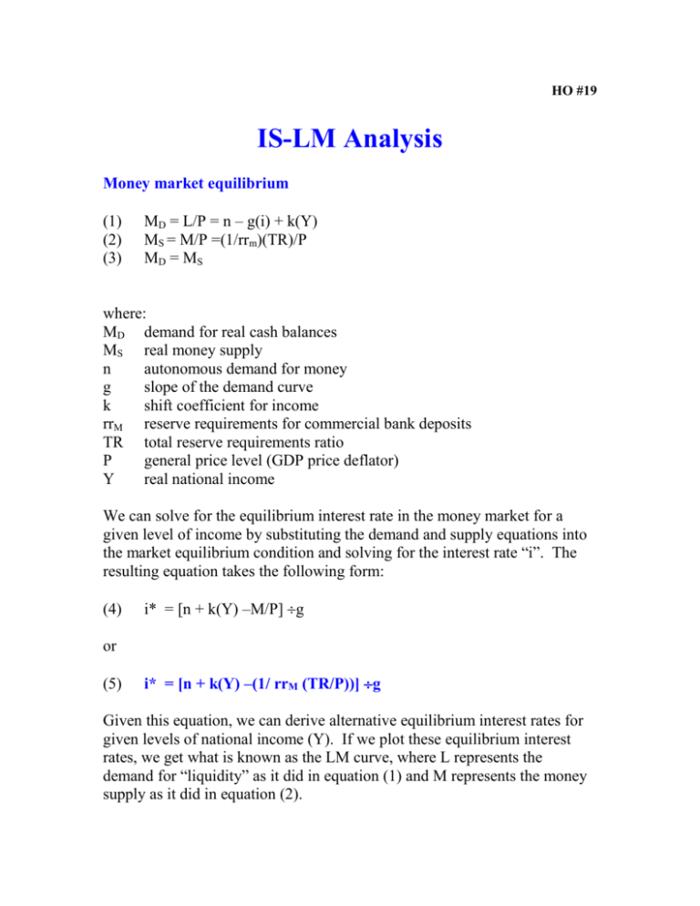
HO #19
IS-LM Analysis
Money market equilibrium
(1)
(2)
(3)
MD = L/P = n – g(i) + k(Y)
MS = M/P =(1/rrm)(TR)/P
MD = MS
where:
MD demand for real cash balances
MS real money supply
n
autonomous demand for money
g
slope of the demand curve
k
shift coefficient for income
rrM reserve requirements for commercial bank deposits
TR total reserve requirements ratio
P
general price level (GDP price deflator)
Y
real national income
We can solve for the equilibrium interest rate in the money market for a
given level of income by substituting the demand and supply equations into
the market equilibrium condition and solving for the interest rate “i”. The
resulting equation takes the following form:
(4)
i* = [n + k(Y) –M/P] g
or
(5)
i* = [n + k(Y) –(1/ rrM (TR/P))] g
Given this equation, we can derive alternative equilibrium interest rates for
given levels of national income (Y). If we plot these equilibrium interest
rates, we get what is known as the LM curve, where L represents the
demand for “liquidity” as it did in equation (1) and M represents the money
supply as it did in equation (2).
LM
i3
i2
i1
Y1
Y2
Y3
Each and every point along the LM curve depicted above represents an
equilibrium in the money market.
Product market equilibrium
(6)
(7)
(8)
(9)
(10)
C = a + b(Y – T)
I = j – f(i)
G = G*
Y=C+I+G
T = h + t(Y)
where:
C
Planned real consumption expenditures
a
Autonomous consumption
b
Marginal propensity to consume
Y
Real national income and product
T
Real government revenue
I
Real planned investment expenditures
j
G
h
t
Autonomous investment
Real government expenditures (* denotes fixed spending)
Tax base
Marginal tax rate
We can solve for the equilibrium level of product or output in the product
market for a given interest rate by substituting the consumption, investment
and government expenditures equations into equation (9) and solve for the
corresponding level of gross domestic product (Y). The resulting equation
takes the following form:
(11) Y* = a + b(Y – T) + j – f(i) + G*
Substituting in the equation for tax revenue (T) into equation (11) and
isolating Y on the left-hand side, we see that:
(12) Y* = [a – b(h) + j + G*]/(1 – b +b(t)) - [f/ (1 – b +b(t))] i
Given this equation, we can derive alternative equilibrium gross domestic
product for given levels of interest rates (i). If we plot these equilibrium
gross domestic product levels, we get what is known as the IS curve, where I
represents the demand for investment expenditures as it did in equation (7)
and S represents the level of savings in the economy, or:
(13)
S=Y–T–C
IS
i3
i2
i1
Y3
Y2
Y1
Each and every point along the IS curve depicted above represents an
equilibrium in the product market.
General equilibrium
We now have two partial equilibriums; one in the money market for given
levels of income and one in the product market for given levels of interest
rates. We can determine the general equilibrium in both markets by
determining where these two curves intersect, or:
IS
LM
iE
YE
This graph suggests that only one interest rate and one level of gross
domestic product satisfies the equilibrium conditions in both markets
simultaneously.
Policy Actions
How does monetary and fiscal policy affect the IS and LM curves?
Expansionary (contractionary) monetary policy will shift the LM curve to
the right (left) while expansionary (contractionary) fiscal policy will shift the
IS curve to the right (left).
Make sure you are comfortable with the implications these changes in policy
will have upon the directional changes for interest rates and gross domestic
product.
Monetary policy actions shift the LM curve and leave the IS curve alone.
Expansionary monetary policy will shift the LM curve to the right, lowering
interest rates and stimulating aggregate demand through investment, jobs
and consumption. Contractionary monetary policy will have exactly the
opposite effects.
IS
LM
LM*
Expansionary
Monetary policy
i
Y
IS
IS*
LM
i
Expansionary
Fiscal policy
Y
Fiscal policy actions shift the IS curve and leave the LM curve alone.
Expansionary fiscal policy will shift the IS curve to the right, stimulating
aggregate demand through increased after tax income and government
spending, but increasing interest rates. Contractionary fiscal policy will
have exactly the opposite effects.
General price level
We can determine the general equilibrium price level in the economy (PE) by
associating the general equilibrium conditions in the last graph with a graph
of the equilibrium in the product market as follows:
IS
LM
iE
YE
AD
PE
AS