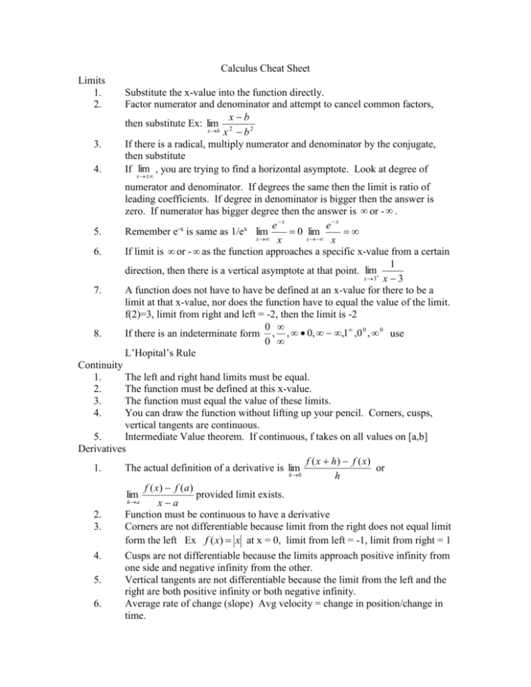
Calculus Cheat Sheet
Limits
1.
2.
3.
4.
5.
6.
7.
8.
Substitute the x-value into the function directly.
Factor numerator and denominator and attempt to cancel common factors,
xb
then substitute Ex: lim 2
x b x  b 2
If there is a radical, multiply numerator and denominator by the conjugate,
then substitute
If lim , you are trying to find a horizontal asymptote. Look at degree of
x  
numerator and denominator. If degrees the same then the limit is ratio of
leading coefficients. If degree in denominator is bigger then the answer is
zero. If numerator has bigger degree then the answer is  or -  .
ex
ex
Remember e-x is same as 1/ex lim
 0 lim

x  x
x   x
If limit is  or -  as the function approaches a specific x-value from a certain
1
direction, then there is a vertical asymptote at that point. lim
x 3 x  3
A function does not have to have be defined at an x-value for there to be a
limit at that x-value, nor does the function have to equal the value of the limit.
f(2)=3, limit from right and left = -2, then the limit is -2
0 
If there is an indeterminate form , ,   0,   ,1 ,0 0 ,  0 use
0 
L’Hopital’s Rule
Continuity
1.
The left and right hand limits must be equal.
2.
The function must be defined at this x-value.
3.
The function must equal the value of these limits.
4.
You can draw the function without lifting up your pencil. Corners, cusps,
vertical tangents are continuous.
5.
Intermediate Value theorem. If continuous, f takes on all values on [a,b]
Derivatives
f ( x  h)  f ( x )
1.
The actual definition of a derivative is lim
or
h 0
h
f ( x)  f (a )
lim
provided limit exists.
ha
xa
2.
Function must be continuous to have a derivative
3.
Corners are not differentiable because limit from the right does not equal limit
form the left Ex f ( x)  x at x = 0, limit from left = -1, limit from right = 1
4.
Cusps are not differentiable because the limits approach positive infinity from
one side and negative infinity from the other.
5.
Vertical tangents are not differentiable because the limit from the left and the
right are both positive infinity or both negative infinity.
6.
Average rate of change (slope) Avg velocity = change in position/change in
time.
7.
8.
9.
10.
11.
12.
13.
14.
15.
16.
Integrals
1.
Know product rule, quotient rule, chain rule (Power trig angle)
d
cos 2 (3x)   sin 2 (3x)  ( cos( 3x))  (3)
Ex
dx
Implicit differentiation (Every y has a y  ) Watch out for product rule. Ex:
x 2  xy  4  2 x  y  xy   0 If given only x-value, subst. to find y value.
Related rates. Derive every variable with respect to time. If a length is
decreasing at t = # then d/dt for that variable is negative.
First derivatve test. Find critical points (anywhere y  = 0 AND any
discontinuity or where the derivative doesn’t exist) y  >0 , then y increasing,
y  < 0 then y decreasing. Max where y  changes from pos. to neg , therefore
y goes from inc. to dec or y  < 0. Min where y  changes from neg. to pos,
therefore y goes from dec. to inc or y  >0.
Second derivative test. Find critical points (anywhere y  = 0 AND any
discontinuity or where the second derivative doesn’t exist) y  >0 , then y
concave up, y  < 0 then y concave down. Points of inflection where
y  changes from pos. to neg or neg to positive or y  changes from increasing
to decreasing .
Logarithmic Differentiation- used mostly with base of x raised to a power of x
or used when there is a rational function with multiple factors in numerator
and/or denominator.
Mean value theorem. F continuous and differentiable on (a,b). Then slope
between 2 points (slope of a secant line between (a,b)) = derivative at some
point c in (a,b) (slope of a tangent line at c). Average rate of change
=instantaneous rate of change.
Know derivatives of polynomials, constants, logartithms, natural logarithms,
exponentials, ex, 6 trig functions, 6 inverse trig functions.
Position, Velocity (derivative of postion), Acceleration (derivative of velocity,
2nd derivative of position).
Derivatives of inverse functions
Fundamental theorem of calculus –
d
dx
u ( x)
 f (t )dt  f (u( x))  u ( x) and
a
b
 f (t )dt  F (a)  F (b)
a
2.
3.
4.
5.
6.
Riemann sums. Right, left and middle. Make rectangles. Width = length of
the subintervals. Height = output value in the table at the middle, left or right.
Trapezoid rule (b-a)/2n*(y0 +2y1+2y2+…+yn)
Trapezoidal approximation - Make trapezoids and add area of each trapezoid.
Integral rules. Separate integrals when there is a sum. Integrate from right to
left then multiply by a negative.
“u” substitutions used to antidifferentiate a chain rule. If you keep the
antiderivative in term of “u”, then you must find the new upper and lower
limits by substituting the original limits into the u substitution.
7.
8.
Integration by parts- used mostly for antidifferentiating a product. uv   vdu
tabular integration is a shortcut
Slope fields – a way of finding the graph of a function without knowing what
the actual function is. Slope fields gives the graphs of an entire family of
functions.
b
9.
10.
11.
12.
13.
14.
15.
16.
17.
18.
19.
20.
a f (t )dt
b
1
Average Value (average y-value)
Function needs
f (t )dt or
ba
b  a a
to be continuous only to apply this calculation.
Euler’s method – another way of getting the graph of a function that has a
differential equation that cannot be solved for y by separation of variables.
Given a diff. equation, an initial point, and x (step size)
x1  current x - value  x , y1  current y - value  diff eq(@curr. point)  x
Repeat procedure to find x2, y2
Separation of varirables for a differential equation. Always put “+C” in right
after antideriving the “x” side. Plug in the initial condition. Solve for “C”
then solve for y with the new “C” value substituted into the problem.
dy
 ky is y  y .0 e kt
Exponential growth: Average Value (average y-value)
dt
dP kP
M  P  M is the carrying capacity. P  M kt

Logistic growth
dt M
1  Ae
Partial Fractions
Position (integral of velocity plug in initial position/condition for C) , Velocity
(integral of acceleration plug in the initial velocity/condition), Acceleration
Final Position = intitial position + displacement (integral of velocity)
Displacement is the integral of velocity for the time values given
Total Distance traveled is the integral of the absolute value of velocity
Integrate a rate to compute the total amount of the quantity (numerator)
Area between curves =
x  value
y  value
xvalue
y  value
 f ( x)  g ( x)dx or  f ( y)  g ( y)dy
x value
21.
Volume =
 ( geometrc cross sectional area) dx
xvalue
22.
Volume of a rotational solid over x-axis = 
x value
 f ( x)
2
dx
2
dy
xvalue
y value
23.
Volume of a rotational solid over y-axis = 
 f ( y)
yvalue
24.
Washer problem over horizontal line BELOW the region =

x  value
 ( f ( x )  L)
xvalue
2
 ( g ( x)  L) 2 dx For f(x) > g(x)
25.
Washer problem over horizontal line ABOVE the region =

x  value
 ( L  g ( x))
2
 ( L  f ( x)) 2 dx For f(x) > g(x)
xvalue
26.
Washer problem over vertical line to the RIGHT of the region =
y  value

 ( L  g ( y))
2
 ( L  f ( y)) 2 dx For f(y) > g(y)
yvalue
27.
Washer problem over vertical line LEFT of the region =
y  value

 ( f ( y )  L)
 ( g ( y )  L) 2 dx For f(y) > g(y)
2
yvalue
b
28.
Length of curve =

a
 dy 
1  
 dx 
30.
a,b are x-values
2
 dx 
Length of curve =  1    c,d are y-values
 dy 
c
If finding the length of curve where the derivative doesn’t exist (cusp, corner,
vertical tangent) Calculate the integral in 2 parts, or solve the equation for x
and use dx/dy. (#29)
d
29.
2
2
 dy 
a 2f ( x) 1   dx  dx
32.
Improper Integrals- replace the  or the limit that is causing a discontinuity
with a variable, then take the limit as this new variable approaches  or the
discontinuity. All other integration techniques can show up with improper
integrals.
33.
Trigonometric substitutions
Parametrics
dy
dy
 dt
1.
First derivative:
dx dx
dt
first derivavtive
2.
Second derivative:
dx
dt
b
31.
Surface Area =
b
3.
Arc Length =

a
Vectors
1.
2
2
 dy 
 dx 
     dt
 dt 
 dt 
Position vector :
x(t , y(t )
2.
Velocity vector
dx dy
,
dt dt
3.
Acceleration vector
d 2x d 2 y
,
dt 2 dt 2
2
4.
Speed is the magnitude of velocity vector =
5.
Displacement =
6.
b
b
a
a
 dy 
 dx 
   
 dt 
 dt 
2
 v1 (t )dt ,  v 2 dt
Total distance Travelled
b
b
a
a
 v(t ) dt  
v1 t 2  v x t 2 dt
Polar Functions
1.
Converting from polar to rectangular/rectangular to polar (Face  walk r.)
2.
x  r cos  , y  r sin 
dy
dy
3.
 d Usually you have to substitute #2 first.
dx dx
d
b
1
4.
Polar Area one function one region:  f ( ) 2 d
2a
b
1
inside 2  outeside 2 d

2a
5.
Polar Area inside one function and outside another
6.
1
1
Polar Area overlapping 2 functions  top 2 d   bottom2 d
2a
2a
b
Series
1.
2.
3.
4.
5.
6.
7.
8.
9.
10.
b
Taylor polynomials general form centered at x = a
Mother functions (centered at x=0)
Maclaurin series (centered at x=0
Integrating and differentiating series (TERM by TERM)
Convergence Tests (PARTING C)
Radius of convergence (R) distance from center that the series can have an
interval of convergence for. x  a  R
Interval of convergence – x values where a series approximation is extremely
close to the function itself. Solve for x in #6 equation or if geometric series
set common ratio <1 and solve for x
a
 f ( x)
Geometric series as a function
1 r
Always check endpoints of series for possible conditional convergence. Plug
endponts of interval of convergence into original series.
La Grange error estimate. If given n terms, look at the max value that can be
obtained form the n+1 term. If the term is already given , just plug in the xvalue that will give you the largest value for that term. If not given the n+1
term, you must compute the max derivative for that term, then plug in the xvalue that would give you the largest overall value for that term.