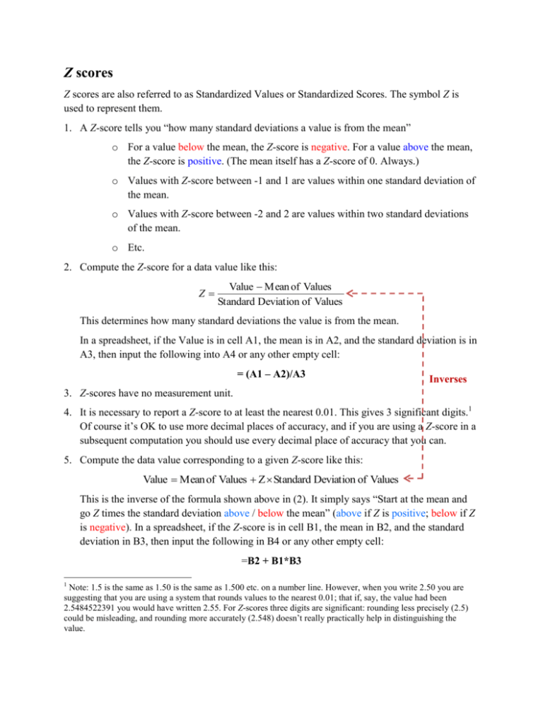
Z scores
Z scores are also referred to as Standardized Values or Standardized Scores. The symbol Z is
used to represent them.
1. A Z-score tells you “how many standard deviations a value is from the mean”
o For a value below the mean, the Z-score is negative. For a value above the mean,
the Z-score is positive. (The mean itself has a Z-score of 0. Always.)
o Values with Z-score between -1 and 1 are values within one standard deviation of
the mean.
o Values with Z-score between -2 and 2 are values within two standard deviations
of the mean.
o Etc.
2. Compute the Z-score for a data value like this:
Z
Value  Mean of Values
Standard Deviation of Values
This determines how many standard deviations the value is from the mean.
In a spreadsheet, if the Value is in cell A1, the mean is in A2, and the standard deviation is in
A3, then input the following into A4 or any other empty cell:
= (A1 – A2)/A3
Inverses
3. Z-scores have no measurement unit.
4. It is necessary to report a Z-score to at least the nearest 0.01. This gives 3 significant digits.1
Of course it’s OK to use more decimal places of accuracy, and if you are using a Z-score in a
subsequent computation you should use every decimal place of accuracy that you can.
5. Compute the data value corresponding to a given Z-score like this:
Value  Mean of Values  Z  Standard Deviation of Values
This is the inverse of the formula shown above in (2). It simply says “Start at the mean and
go Z times the standard deviation above / below the mean” (above if Z is positive; below if Z
is negative). In a spreadsheet, if the Z-score is in cell B1, the mean in B2, and the standard
deviation in B3, then input the following in B4 or any other empty cell:
=B2 + B1*B3
1
Note: 1.5 is the same as 1.50 is the same as 1.500 etc. on a number line. However, when you write 2.50 you are
suggesting that you are using a system that rounds values to the nearest 0.01; that if, say, the value had been
2.5484522391 you would have written 2.55. For Z-scores three digits are significant: rounding less precisely (2.5)
could be misleading, and rounding more accurately (2.548) doesn’t really practically help in distinguishing the
value.
6. Even without seeing a data set, you should guess that
o about 68% of the data has Z-score between -1 and 1,
o about 95% of the data has Z-score between -2 and 2,
o almost all of the data has Z-score between -3 and 3.
These reflect a generalization obtained from empirical observation of many data sets. For
distributions that are Normal (bell-shaped) or nearly Normal, these three statements are quite
accurate.
It is uncommon to have a Z-score outside of -3 to 3; fairly rare to see one outside of -4 to 4.
7. If you have a data set and use its mean and standard deviation to compute a Z-score for every
value in the set, then the mean of all the Z-scores is 0 and the standard deviation of all the Zscores is 1. Always. This happens with every data set.
8. Z-scores outside of -10 to 10 cannot occur for more than 1% of the values in a data set. (This
is a mathematical fact.) In practice Z-scores larger than 4 (positive or negative) are rare, and
getting rarer as the magnitude of the Z-score increases.
9. The shape of the distribution of Z-scores is identical to the shape of the distribution of data.
10. If two distributions have the same shape, values from each distribution which match on Zscores also match on percentile rank.
This implies two things.
o The idea is that stating values in terms of Z-scores puts every data set on an
identical scale. Consider for instance data measured in inches (heights of adult
men). If the data are all changed to centimeters, by multiplying each value by 2.54
in/cm, then of course the mean and standard deviation are converted the same
way. A histogram of the data is virtually the same whether the horizontal axis is
labeled in inches or in centimeters. Z-scores will be the same whether computed
from the inches version or the centimeters version. And similarly, while the
horizontal axis of the histogram of Z-scores is now on a different scale, the shape
of the histogram is identical.2
o Distributions for two different data sets, measured on different scales, can be
made commensurate by converting each set to Z-scores. This requires that the two
sets have distributions with identical shapes.
2
Departures from this are due only to smart software, which will attempt to round histogram bin endpoints to
convenient values. While 60 inches is identical to 152.4 cm, 60 in is nice for easy reading on a graph while 152.4 cm
is not; software will probably bin differently for the two situations.
Data in Patient Waiting Time tab in Continuous Data
Histograms for the data in units of minutes, hours, and the unit-free Z-scores.
Mean = 92.82 minutes
9
SD = 32.82 minutes
8
Outlier (Max) = 201 minutes
= 3.30
# of Patients
Z = (201 – 92.82) / 32.82
7
6
5
4
3
2
1
0
40
80
120
160
Waiting Times (minutes)
200
Mean = 1.547 hours
9
SD = 0.547 hours
8
Outlier (Max) = 3.35 hours
= 3.30
# of Patients
Z = (3.35 – 1.547) / 0.547
7
6
5
4
3
2
1
0
0.5
1.0
1.5
2.0
2.5
Waiting Times (hours)
3.0
3.5
-2
-1
0
1
2
Waiting Times (Z-scores)
3
4
Mean = 0.00
9
SD = 1.00
8
Outlier (Max) = 3.30
# of Patients
7
6
5
4
3
2
1
0
Data in Jan Temps tab in Continuous Data
Histograms for the data in units of degrees Farenheit, Centigrade, and the unit-free Z-scores.
Mean = 23.98 F
25
SD = 4.68 F
Min = 13.6 F
= -2.22
Max = 35.8 F
Z = (35.8 – 23.98) / 4.68
Number of Januaries
Z = (13.6 – 23.98) / 4.68
20
15
10
5
= 2.53
0
Mean = -4.46 C
15
18
21
24
27
30
January Mean Temperature (F)
33
36
30
SD = 2.60 C
25
Z = (-10.22 – -4.46) / 2.60
= -2.22
Max = 2.11 C
Number of Januaries
Min = -10.22 C
20
15
10
Z = (2.11 – -4.46) / 2.60
5
= 2.53
0
Mean = 0
-10
-8
-2.4
-1.6
-6
-4
-2
January Mean Temperature (C)
0
2
35
SD = 1
30
Max = 2.53
Number of Januaries
Min = -2.22
25
20
15
10
5
0
-0.8
0.0
0.8
1.6
January Mean Temperature (Z-score)
2.4
3.2
Exercises
There’s no harm in identifying the units of observation and the variable in each exercise.
1. SAT Math scores for college applicants have mean 543 and standard deviation 110.
a) Find the Z-scores for applicants with the following SAT Math scores:
300
400
500
600
700
800
b) Find the SAT Math scores for applicants with the following Z-scores:
-2.09 -1.30 -0.39 0.52
1.43
2.34
c) Compare inputs and outputs from parts (a) and (b).
2. Find a data set. Any data set will do. Compute the mean and standard deviation. Then obtain
the Z-score for each value in the set.
a) Determine the mean of the Z-scores.
b) Determine the standard deviation of the Z-scores.
c) What is the largest negative Z-score? (This goes with the minimum.) What is the largest
positive Z-score? (This goes with the maximum.)
Now repeat this for as many other data sets as you like…enough to convince yourself that

The mean of all Z-scores is always 0.

The standard deviation of all Z-scores is always 1.

Z-scores outside -3 to 3 are pretty uncommon (at least for real data sets); Z-scores
outside -4 to 4 are quite rare.
3. Dan has collected data on the amount of time people exercise per week. He obtains a Z-score
for each person’s time. What are the mean and standard deviation of this collection of Zscores?
4. Nationwide, statisticians with a master’s degree have mean salary $111K with standard
deviation $22K. Make some guesses…
a) 68% of these people earn between $_____K and $_____K .
b) 95% of these people earn between $_____K and $_____K .
c) How many standard deviations from the mean is a salary of $82K? How about $200K?
d) What is the salary of such a person who is 3.50 standard deviations below the mean?
How about one who is 1.43 standard deviations above the mean?
5. Nationwide, those with an MBA have mean salary $124K with standard deviation $61K.
Make some more guesses…
a) ___% of these people earn between $63K and $185K .
What can you say about the Z-scores for those with salary between $63K and $185K?
b) ___% of these people earn between $2K and $246K .
What can you say about the Z-scores for those with salary between $2K and $246K?
c) How many standard deviations from the mean is a salary of $82K? How about $200K?
d) What is the salary of such a person who is 3.50 standard deviations below the mean?
How about one who is 1.43 standard deviations above the mean?
e) Chris, an MBA, claims a salary that is 12 standard deviations above the mean. What
would such a salary be? Is such a salary possible? Is it common?
6. Daily water consumption at a pet shop has mean 1500 gallons with standard deviation 325
gallons.
a) Write two statements that are educated guesses about the distribution.
i.
On ___% of days water consumption is between _____ and _____ gallons.
ii.
On ___% of days water consumption is between _____ and _____ gallons.
b) What’s the consumption, in gallons, on a day for which the Z-score is 1.24?
c) What’s the consumption, in gallons, for a day where consumption is 2.40 standard
deviations below the mean consumption?
7. A company’s monthly travel costs in the United States have mean $40,525 and standard
deviation $8,145.
a) Find the Z-score for a month in which the cost of travel is $70,000. Would so high an
expense be common?
b) In one month, the cost was 2.42 standard deviations above the mean. What was the cost?
c) What is the expense for a month with Z-score of -1.75?
The company does business in the U.S. but is based in Europe. The accounting is done in
Euros (not dollars).
d) In Euros, what are the mean and standard deviation of the monthly travel costs?
e) Find the Z-score for a month in which the cost is 52,808 Euros. Compare to your answer
in part (a).
8. Take a look at the Cloud Seeding Study.
a) Determine one Z-score for the maximum rainfall amount for the seeded clouds, and
another for the unseeded clouds. These are fairly large, and fairly close, suggesting that
relative to their distributions, these amounts are fairly similar. (In fact the two values
share a percentile rank of 100 within their respective data sets.)
b) For each data set, determine the rainfall amount corresponding to a Z-score of -0.75? Is
such a Z-score meaningful for this data? Why not? How can a Z-score of 3.50 be
possible, but not one of -0.75?
Solutions
1. Variable: SAT Math scores. Units: college applicants.
have mean 543 and standard deviation 110.
a) -2.21, -1.30, -0.39, 0.52, 1.43, 2.34
b) 300, 400, 500, 600, 700, 800.
c) The inputs to (b) are the outputs of (a); the inputs of (a) are the outputs of (b).
2. “Answers” are in the question.
3. Variable: amount of exercise per week. Units: people. The mean is 0; the standard deviation
is 1.
4.
Units = people with master’s degree in statistics. Variable = salary.
a) 68% of these people earn between $89K and $133K .
b) 95% of these people earn between $67K and $155K .
c) $82K is 1.32 standard deviations below the mean? $200K is 4.05 standard deviations
above the mean.
d) If Z = -3.50 then the salary is 111 – 3.5(22) = $34K. If Z = 1.43 then the salary is
111 + 1.43(22) = $142.46K.
5.
Units = people with MBAs. Variable = salary.
a) 68% of these people earn between $63K and $185K . The Z-scores are between -1 and 1.
b) 95% of these people earn between $2K and $246K . The Z-scores are between -1 and 1.
c) $82K: Z = -0.69, so 0.69 standard deviations below the mean. $200K: 1.25 standard
deviations above the mean.
d) A person who is 3.50 standard deviations below the mean has salary
124 – 3.5(61) = -$89.5K, which cannot occur. One who is 1.43 standard deviations above
the mean has salary $211.23K.
e) $856K – which is possible (and certainly does occur) but uncommon.
6.
Units = days. Variable = water consumption.
a) Both are guesses…
i.
On 68% of days water consumption is between 1175 and 1825 gallons.
ii.
On 95% of days water consumption is between 850 and 2150 gallons.
b) 1903 gallons.
c) 720 gallons.
7. Units = months. Variable = travel cost.
a) 3.62. This would be uncommon (it’s more than 3.5 standard deviations above the mean).
b) $60236.
c) $26271.
d) The answer depends on the conversion rate. As this solution is created, that rate is 0.7544
Euros per dollar. So the mean is 0.7544(40525) = 30,572 Euros; the standard deviation is
0.7544(8145) = 6,145 Euros.
e) 3.62. This is identical to the result from (a) because Z-scores don’t depend on the
measurement units. Using the mean and standard deviation from d: (52,808 – 30572) /
6145 = 3.62. This happens even if the conversion rate is different from 0.7544 – it
happens no matter what the conversion rate is.
8. Units = clouds. Variable = rainfall.
a) Seeded: 3.54. Unseeded: 3.65.
b) Seeded: -46.1 acre-feet. Unseeded: -47.8 acre-feet. Negative rainfall is impossible. A Zscore of 3.50 be possible, but not one of -0.75, because this distribution is highly right
skewed, with an outlier to the right.