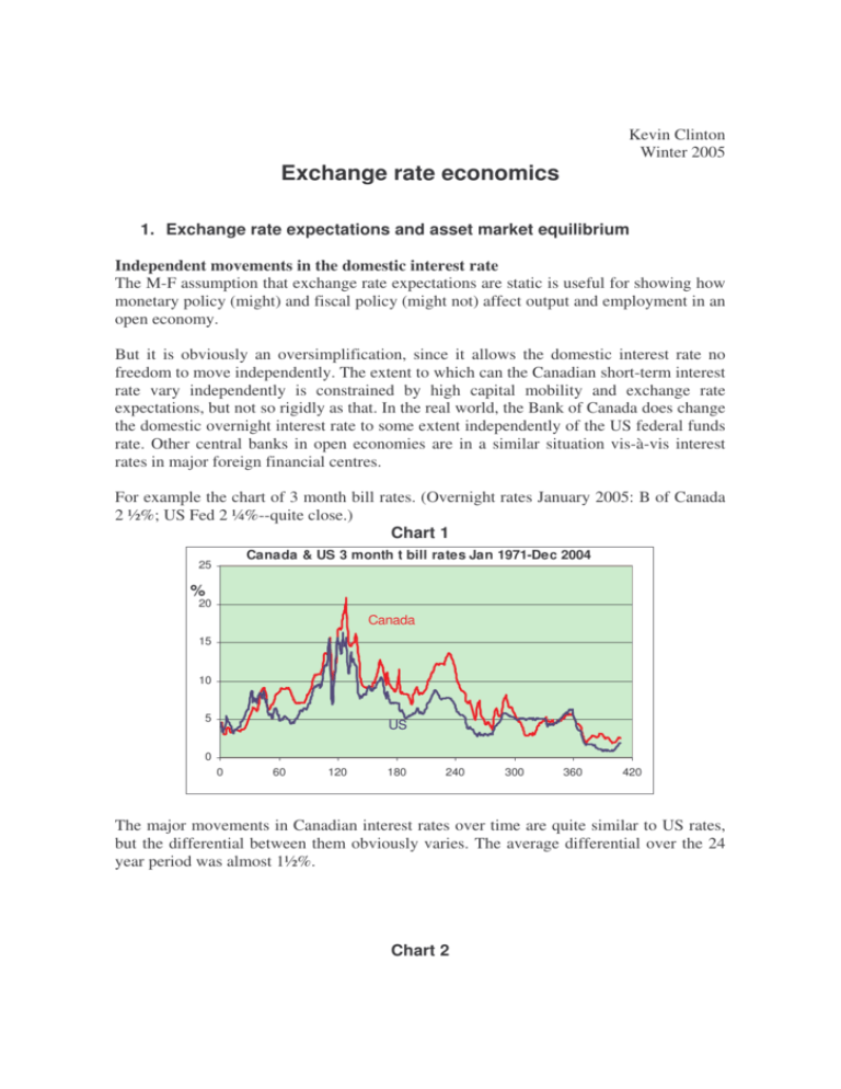
Kevin Clinton
Winter 2005
Exchange rate economics
1. Exchange rate expectations and asset market equilibrium
Independent movements in the domestic interest rate
The M-F assumption that exchange rate expectations are static is useful for showing how
monetary policy (might) and fiscal policy (might not) affect output and employment in an
open economy.
But it is obviously an oversimplification, since it allows the domestic interest rate no
freedom to move independently. The extent to which can the Canadian short-term interest
rate vary independently is constrained by high capital mobility and exchange rate
expectations, but not so rigidly as that. In the real world, the Bank of Canada does change
the domestic overnight interest rate to some extent independently of the US federal funds
rate. Other central banks in open economies are in a similar situation vis-à-vis interest
rates in major foreign financial centres.
For example the chart of 3 month bill rates. (Overnight rates January 2005: B of Canada
2 ½%; US Fed 2 ¼%--quite close.)
Chart 1
Canada & US 3 month t bill rates Jan 1971-Dec 2004
25
%
20
Canada
15
10
5
US
0
0
60
120
180
240
300
360
420
The major movements in Canadian interest rates over time are quite similar to US rates,
but the differential between them obviously varies. The average differential over the 24
year period was almost 1½%.
Chart 2
Canada - US 3 month t bill differential Jan 1971-Dec 2004
6.00
%
4.50
3.00
1.50
0.00
0
60
120
180
240
300
360
420
-1.50
-3.00
A realistic model allows some interest rate independence in the short-run, but not in the
long run. For this, we have to modify the static expectations in the M-F model.
Dornbusch assumed rational expectations for the exchange rate. That is, the expected
value of the exchange rate is the long-run equilibrium value.
Uncovered interest parity
With perfect capital mobility, the domestic interest rate is equal to the foreign rate minus
the expected increase in the exchange value of the currency:
rt = r*t - Et∆et ,
where Et∆εt is the expected percentage appreciation of the domestic currency.1 This may
be written as
rt = r*t + Et(et+1) - et.
(1)
where Et(et+1) is the expected value, in period t, of e in t+1.
Equation (1) is known as uncovered interest parity (UIP). The expected rate of return is
the same, adjusted for expected changes in the exchange rate, regardless of currency. UIP
holds in the special case of the M-F model, with Et∆et = 0.
In effect, et (non-italic) is the logarithm of the exchange rate, e (italic), and ∆et is the percentage
change in e.
1
2
Rapid asset price adjustment
The short-run interest rate is set by the central bank, and the exchange rate adjusts
instantly—see chart 5. Financial asset markets clear continuously. (The output price
level, in contrast, is sticky—does not instantly jump from one LR equilibrium position to
the next, but moves in steps over a period of time.)
Chart 3
Exchange rate: US$ per C$ Jan 1971-Dec 2004
1
0.9
0.8
0.7
0.6
0
60
120
180
240
300
360
420
We can draw an asset market equilibrium line, AA, in (e, r) space from which there are no
deviations, even in the short run. The asset market equilibrium line slopes down, showing
the intuitive feature that an increase in the domestic interest rate is associated with a
strengthened currency.
3
Figure 1
General equilibrium: asset and output markets
r
IS: FE
equilibrium
AA: asset market
equilibrium
r2
r1
e1
e
e2
At an interest rate above r1, say r2, asset market equilibrium requires that the exchange
rate appreciate, to e2 in the chart. People expect the exchange rate to return to the longrun equilibrium value e1. That is, they expect e to fall. With UIP, the expected decrease in
e just compensates for the higher domestic interest rate.
Example A 100 basis point (one percentage point) increase in r for one period causes e to
rise one per cent. Investors expect it to fall back to its equilibrium value next period. The
expected exchange loss is equal to the domestic-foreign interest rate differential.
Evidence According to the theory, the Canada-US interest differential and the C$/US$
exchange rate should be positively correlated. The chart below shows some correlation,
particularly since the mid-1980s, but it is quite loose.
Chart 4
US $/C$ ra te a nd t bill spre a d Ja n 1971-De c 2004
1.05
e xch a n g e ra te
t b ill s p re a d (s ca le d )
0.95
0.85
0.75
0.65
0.55
0
60
120
180
240
300
360
420
4
The problem with interpreting data is that in the real world many things happen at the
same time. There is not a simple experiment in which the central bank shocks the interest
rate to see what happens—monetary policy is itself responding to economic events,
including sometimes changes in the exchange rate (e.g. 1992, 1995, and 1998). So we
have causality going both ways—the identification problem in econometrics. However
we can see the effect of the tight money policy of the late 1980s and early 90s in both the
interest rate differential (strongly up) and e (up too). Likewise, the easing of monetary
policy, after the inflation rate was brought down to the target rate of 2%, later in the
1990s, is evident in the steep (if uneven) decline in the interest rate, and the drop in e to
record lows.
2. Monetary policy
Figure 2
Monetary contraction—increased interest rate
r
IS: FE
equilibrium
AA: asset market
equilibrium
r2
r1
e1
e2
e
Temporary monetary contraction
The central bank raises the interest rate, from r0 to r1, for 1 year.
For UIP (equation 1) to hold, e must immediately rise to a higher level, e2, such that its
expected depreciation afterwards, back to the long-run equilibrium e1, exactly offsets the
interest differential:
E1(et+2) - e2 = e1 - e2 = r1 - r0.
The asset market equilibrium line AA has a negative slope: in increase in the short-term
interest differential requires the exchange rate to jump immediately, to the point that
investors think that it will now decline at a rate that offset the interest differential.
Moreover, since asset prices are fully flexible, the asset market is always in equilibrium,
so the path to long-run equilibrium is along AA.
5
Exchange rate flexibility, with non-static expectations, allows monetary policy to affect r
as well as e, whereas it affects only e in the M-F model.
In the example the increase in both r and e is deflationary: output falls below potential.
The monetary contraction reduces output. The price level would eventually fall if the
tight policy continued, but in the short run it stays constant (price level stickiness).
Figure 3
Temporary monetary contraction: paths of interest and exchange rates
r2
r1
0
1
2
year
3
e1
0
1
2
3
year
A general implication of all flexible exchange rate models is that there is a positive
correlation between the real exchange value of the currency and the real interest
differential. In a situation where inflations rates are low and stable, this implies a positive
correlation between the exchange rate and the nominal interest differential.
6
Permanent monetary contraction
In the long run, a permanent monetary contraction results in no change in output, and a
decrease in both the money stock and the price level (long-run classical monetary
neutrality). In the short-run, however, because of sticky prices for goods and labour, the
price level does not drop immediately, but adjusts over time, and output declines.
Figure 4
Permanent monetary contraction: paths of output & price level
y1
y2
0
2
4
0
2
4
0
2
4
year
6
p1
p3
year
6
Inflation
∆p
0
6
year
In the long run the price level will fall by the same percentage as the money stock.
During the adjustment period there is deflation (negative inflation).
7
Figure 5
Permanent monetary contraction: paths of interest & exchange rate
r2
r1
rate E
0
2
4
0
2
4
year
6
Ε2
E3
E1
6
year
The interest rate rises, causing deflation in the goods market. As the price level falls, the
value of the real money stock rises (nominal money supply is constant at the new higher
level), which allows the interest rate to decline. In the long run the decrease in the price
level restores the real value of money supply to its initial equilibrium level, and the
interest rate also returns to initial equilibrium.
The initial equilibrium nominal exchange rate is E1. After the increase in the money
supply, the long-run equilibrium is E3. Constancy of the real equilibrium exchange rate
(purchasing power parity) requires that in the long run the nominal exchange rate E rise
by the same percentage that the price level falls.
Exchange rate overshooting
With the permanent decrease in the money stock (and price level) the exchange rate
depreciates more in the short-run than in the long run. This is because of uncovered
interest parity, allied to the expectation that the exchange rate will eventually reach
equilibrium level e3.
Hence the name: Dornbusch exchange-rate overshooting model.
Conclusion
Monetary policy has substantial effects on output and prices in an open economy with a
floating exchange rate. The change in the exchange rate (the external channel) reinforces
the policy change in the interest rate (the domestic channel of transmission of monetary
policy).
8
3. Other determinants of Canadian exchange rate
Commodity prices
Chart 4
Commodity prices and US$/C$ rate
Indexes of commodity prices
C$
The positive correlation between the C$ (thick line), and the indexes of commodity prices
reflects Canada’s position as a large exporter of resource-based output.
Relative international price levels: Purchasing Power Parity
The principle of purchasing power parity (PPP) says that in the long run exchange rate
movements reflect movements in relative price levels. In the simplest version, PPP
implies that the nominal exchange rate moves exactly to offset differing price level
movements: the real exchange rate is constant. Competition and arbitrage of goods across
borders ensure some such tendency. Inflation does weaken a currency.
However, other things, which vary over time, affect the real equilibrium value of a
currency. In fact, movements in the real (price level adjusted) US$/C$ exchange rate
e = E * PCAN/PUS
shows somewhat more stability over time than the nominal rate E, which is weak
evidence of PPP. But it does not show the convergence to a constant value implied by the
simple version of PPP.
9
4. Contrast of regimes: flexible versus fixed exchange rate
A fixed exchange rate regime implies a very different monetary policy environment from
a flexible exchange rate.
Fixed exchange rate regime
Monetary policy
There is no independent monetary policy, since the interest rate is fixed in the rest of the
world, and the nominal exchange rate cannot change.
Fiscal policy
Since neither the interest rate nor the exchange rate can change, expansionary fiscal
policy has strong short-run output effects. There is no offset from currency appreciation
as in the floating regime, or from interest rate increases as in the closed economy case.
However, this also means that there are large implications for foreign indebtedness,
which grow over time. Fixed exchange rate regimes often collapse in a crisis when
foreign debt burdens become excessive.
Adjustment to exogenous real shocks
The processes of adjustment following shocks to foreign demand, etc., are much slower
under a fixed exchange rate. Reason: the exchange rate can jump immediately to a new
equilibrium, whereas price levels adjust relatively slowly over time.
For example, following a sharp increase in raw materials prices, the nominal C$ usually
appreciates promptly. This helps keep the economy in equilibrium—the increased value
of the C$ releases resources for use in the booming industries. Under a fixed regime, the
required real appreciation of the C$ has to occur through domestic inflation—which takes
time.
A downside shock to demand would involve a particularly prolonged and painful
adjustment period—a recession—because the overall domestic wage and price level is
particularly inflexible in the downward direction.
Volatility of exchange rates
Some economists worry about the volatility of floating exchange rates. Exchange rates
often vary for no apparent reason at all. Sometimes it is difficult to see a correlation with
economic fundamentals. There is a lot of froth in financial markets, exchange markets
included. However:
1. There is no evidence that weekly or monthly volatility has any significant
macroeconomic effects at all.
2. The broad movements in the C$, over years, have been in an equilibrating direction—
e.g. the dismal 1990s would have been even more dismal if the C$ had not depreciated
10
20% or more. And with the strong demand for Canadian exports, and high commodity
prices, over the past couple of years, the rise in the C$ has held inflation in check.
Monetary unions
These are fixed exchange rate regions par excellence—there is only one money.
Examples: Canada, the euro area.
In Canada monetary union issues arise in 3 contexts:
•
•
•
Provincial fiscal policy—in a large province fiscal expansion might increase
provincial output in the short run (the fixed exchange rate case) but it has a
negative impact on other provinces through effects on interest rates—e.g. Ontario
1985-95. “Beggar thy neighbour” policy.
Debate about monetary union with US. Lower transactions costs, and more trade,
versus adjustment problems.
Quebec secession scenarios—the PQ has debated these regimes: the C$; the US$;
and a Q$?
Re the euro area, note:
•
just one monetary policy for the whole area—too soon to judge how effective this
is, but there are obvious teething problems at least
•
the Maastrich Stability and Growth Pact puts a 3% limit on government
deficit/GDP ratio—an effort to stop the beggar-thy-neighbour fiscal policy, which
is a risk in a currency union. Again, not clear yet whether this is effective.
11