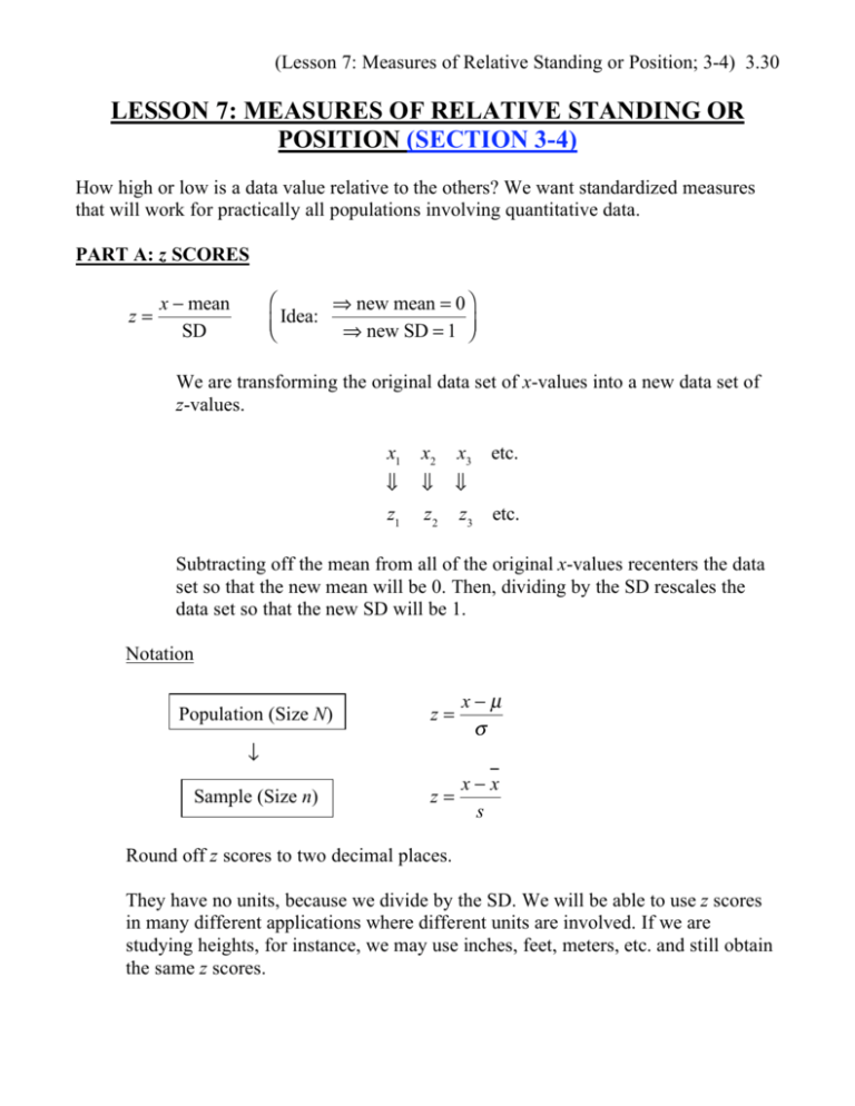
(Lesson 7: Measures of Relative Standing or Position; 3-4) 3.30
LESSON 7: MEASURES OF RELATIVE STANDING OR
POSITION (SECTION 3-4)
How high or low is a data value relative to the others? We want standardized measures
that will work for practically all populations involving quantitative data.
PART A: z SCORES
z=
new mean = 0 Idea:
new SD = 1 x mean
SD
We are transforming the original data set of x-values into a new data set of
z-values.
x1
x2
x3
etc.
z1
z 2 z3
etc.
Subtracting off the mean from all of the original x-values recenters the data
set so that the new mean will be 0. Then, dividing by the SD rescales the
data set so that the new SD will be 1.
Notation
Population (Size N)
z=
xμ
z=
xx
s
Sample (Size n)
Round off z scores to two decimal places.
They have no units, because we divide by the SD. We will be able to use z scores
in many different applications where different units are involved. If we are
studying heights, for instance, we may use inches, feet, meters, etc. and still obtain
the same z scores.
(Lesson 7: Measures of Relative Standing or Position; 3-4) 3.31
z Score Rule of Thumb for “Unusual” Data Values
Data values whose corresponding z scores are either less than 2 or greater
than 2 (i.e., z < 2 or z > 2 ) are often considered “unusual.”
In other words, data values that are more than 2 SDs from the mean are
often considered “unusual.”
Think About It: How would you feel if your instructor tells you that your z score
for the test you just took was 2.31 ?
Example
Two statistics classes take different tests.
The mean and SD for Class 1 are: μ1 = 55 points , 1 = 5 points .
The mean and SD for Class 2 are: μ2 = 60 points , 2 = 10 points .
In which class is a score of 70 points more impressive?
Solution
Find the corresponding z scores for 70 points in the two classes.
Class 1:
Class 2:
70 55
5
= 3.00
z=
70 60
10
= 1.00
z=
A score of 70 points is more impressive in Class 1; in fact, it is “unusually”
high in that class.
(Lesson 7: Measures of Relative Standing or Position; 3-4) 3.32
Note: If we assume normality in both classes, we have:
PART B: FRACTILES, OR QUANTILES
We will look at three types of these.
Percentiles
Example
Because 92% of the scores lie below 85 points, we can say that the
92nd percentile of the data is 85: P92 = 85 points .
(Lesson 7: Measures of Relative Standing or Position; 3-4) 3.33
Deciles
Think: Dimes.
1st decile = D1 = P10
2 nd decile = D2 = P20
9 th decile = D9 = P90
Quartiles
Think: Quarters.
1st quartile = Q1 = P25
2 nd quartile = Q2 = P50
3rd quartile = Q3 = P75
( Median )
(Lesson 8: Boxplots; also 3-4) 3.34
LESSON 8: BOXPLOTS (ALSO SECTION 3-4)
The Five-Number Summary can be represented graphically as a boxplot, or box-andwhisker plot.
Boxplots can help us compare different populations, such as men and women.
See the last page of the MINITAB handout.