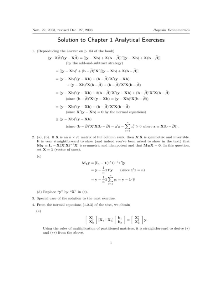
Nov. 22, 2003, revised Dec. 27, 2003
Hayashi Econometrics
Solution to Chapter 1 Analytical Exercises
1. (Reproducing the answer on p. 84 of the book)
e 0 (y − Xβ)
e = [(y − Xb) + X(b − β)]
e 0 [(y − Xb) + X(b − β)]
e
(y−Xβ)
(by the add-and-subtract strategy)
e 0 X0 ][(y − Xb) + X(b − β)]
e
= [(y − Xb)0 + (b − β)
e 0 X0 (y − Xb)
= (y − Xb)0 (y − Xb) + (b − β)
e + (b − β)
e 0 X0 X(b − β)
e
+ (y − Xb)0 X(b − β)
e 0 X0 (y − Xb) + (b − β)
e 0 X0 X(b − β)
e
= (y − Xb)0 (y − Xb) + 2(b − β)
e 0 X0 (y − Xb) = (y − Xb)0 X(b − β))
e
(since (b − β)
e 0 X0 X(b − β)
e
= (y − Xb)0 (y − Xb) + (b − β)
(since X0 (y − Xb) = 0 by the normal equations)
≥ (y − Xb)0 (y − Xb)
e 0 X0 X(b − β)
e = z0 z =
(since (b − β)
n
X
i=1
e
zi2 ≥ 0 where z ≡ X(b − β)).
2. (a), (b). If X is an n × K matrix of full column rank, then X0 X is symmetric and invertible.
It is very straightforward to show (and indeed you’ve been asked to show in the text) that
MX ≡ In − X(X0 X)−1 X0 is symmetric and idempotent and that MX X = 0. In this question,
set X = 1 (vector of ones).
(c)
M1 y = [In − 1(10 1)−1 10 ]y
1
= y − 110 y
(since 10 1 = n)
n
n
1 X
=y− 1
yi = y − 1· y
n i=1
(d) Replace “y” by “X” in (c).
3. Special case of the solution to the next exercise.
4. From the normal equations (1.2.3) of the text, we obtain
(a)
X01
X02
.
[X1 .. X2 ]
b1
b2
=
X01
X02
y.
Using the rules of multiplication of partitioned matrices, it is straightforward to derive (∗)
and (∗∗) from the above.
1
(b) By premultiplying both sides of (∗) in the question by X1 (X01 X1 )−1 , we obtain
X1 (X01 X1 )−1 X01 X1 b1 = −X1 (X01 X1 )−1 X01 X2 b2 + X1 (X01 X1 )−1 X01 y
⇔ X1 b1 = −P1 X2 b2 + P1 y
Substitution of this into (∗∗) yields
X02 (−P1 X2 b2 + P1 y) + X02 X2 b2 = X02 y
⇔
X02 (I − P1 )X2 b2 = X02 (I − P1 )y
⇔ X02 M1 X2 b2 = X02 M1 y
⇔
Therefore,
X02 M01 M1 X2 b2 = X02 M01 M1 y
e0 X
e
e 0 e.
⇔ X
2 2 b2 = X2 y
(since M1 is symmetric & idempotent)
e0 X
e −1 X
e0 y
b2 = ( X
2 2)
2e
e
e
e
e0 X
(The matrix X
2 2 is invertible because X2 is of full column rank. To see that X2 is of full
e
column rank, suppose not. Then there exists a non-zero vector c such that X2 c = 0. But
e 2 c = X2 c − X1 d where d ≡ (X0 X1 )−1 X0 X2 c. That is, Xπ = 0 for π ≡ −d . This is
X
1
1
c
..
a contradiction because X = [X1 . X2 ] is of full column rank and π 6= 0.)
(c) By premultiplying both sides of y = X1 b1 + X2 b2 + e by M1 , we obtain
M1 y = M1 X1 b1 + M1 X2 b2 + M1 e.
e ≡ M1 y, the above equation can be rewritten as
Since M1 X1 = 0 and y
e = M1 X2 b2 + M1 e
y
e 2 b2 + M1 e.
=X
M1 e = e because
M1 e = (I − P1 )e
= e − P1 e
= e − X1 (X01 X1 )−1 X01 e
=e
(since X01 e = 0 by normal equations).
(d) From (b), we have
e0 X
e −1 X
e0 y
b2 = (X
2 2)
2e
0
−1
0
e X
e 2 ) X M0 M1 y
= (X
2
2
1
e0 X
e −1 X
e 0 y.
= (X
2 2)
2
e 2 . The residual
Therefore, b2 is the OLS coefficient estimator for the regression y on X
vector from the regression is
e 2 b2 = (y − y
e 2 b2 )
e ) + (e
y−X
y−X
e 2 b2 )
= (y − M1 y) + (e
y−X
= (y − M1 y) + e
= P1 y + e.
2
(by (c))
This does not equal e because P1 y is not necessarily zero. The SSR from the regression
e 2 can be written as
of y on X
e 2 b2 )0 (y − X
e 2 b2 ) = (P1 y + e)0 (P1 y + e)
(y − X
= (P1 y)0 (P1 y) + e0 e
(since P1 e = X1 (X01 X1 )−1 X01 e = 0).
This does not equal e0 e if P1 y is not zero.
e 2 b2 + e. So
e=X
(e) From (c), y
e 2 b2 + e)0 (X
e 2 b2 + e)
e0 y
e = (X
y
0
e0 X
e
e 2 e = 0).
= b02 X
(since X
2 2 b2 + e e
e0 X
e −1 X
e 0 y, we have b0 X
e0 e
e 0 X2 (X02 M1 X2 )−1 X2 y
e.
Since b2 = (X
2 2)
2
2 2 X2 b2 = y
b
e on X1 . Then
(f) (i) Let b1 be the OLS coefficient estimator for the regression of y
b 1 = (X0 X1 )−1 X0 y
b
1
1e
= (X01 X1 )−1 X01 M1 y
= (X01 X1 )−1 (M1 X1 )0 y
=0
(since M1 X1 = 0).
b 1 )0 (e
b1) = y
e0 y
e.
So SSR1 = (e
y − X1 b
y − X1 b
e 2 equals e by (c), SSR2 = e0 e.
e on X
(ii) Since the residual vector from the regression of y
e on X1 and
(iii) From the Frisch-Waugh Theorem, the residuals from the regression of y
e 2 ). So SSR3 = e0 e.
e (= y
e ) on M1 X2 (= X
X2 equal those from the regression of M1 y
5. (a) The hint is as good as the answer.
b the residuals from the restricted regression. By using the add-and-subtract
(b) Let b
ε ≡ y−Xβ,
strategy, we obtain
b = (y − Xb) + X(b − β).
b
b
ε ≡ y − Xβ
So
b 0 [(y − Xb) + X(b − β)]
b
SSRR = [(y − Xb) + X(b − β)]
b 0 X0 X(b − β)
b
= (y − Xb)0 (y − Xb) + (b − β)
(since X0 (y − Xb) = 0).
But SSRU = (y − Xb)0 (y − Xb), so
b 0 X0 X(b − β)
b
SSRR − SSRU = (b − β)
= (Rb − r)0 [R(X0 X)−1 R0 ]−1 (Rb − r)
= λ0 R(X0 X)−1 R0 λ
0
0
−1
=b
ε X(X X)
=b
ε0 Pb
ε.
0
Xb
ε
b from (a))
(using the expresion for β
(using the expresion for λ from (a))
b = R0 λ)
(by the first order conditions that X0 (y − Xβ)
(c) The F -ratio is defined as
F ≡
(Rb − r)0 [R(X0 X)−1 R0 ]−1 (Rb − r)/r
s2
3
(where r = #r)
(1.4.9)
Since (Rb − r)0 [R(X0 X)−1 R0 ]−1 (Rb − r) = SSRR − SSRU as shown above, the F -ratio
can be rewritten as
(SSRR − SSRU )/r
s2
(SSRR − SSRU )/r
=
e0 e/(n − K)
(SSRR − SSRU )/r
=
SSRU /(n − K)
F =
Therefore, (1.4.9)=(1.4.11).
6. (a) Unrestricted model: y = Xβ + ε, where



y1
1 x12
 .. 
 ..
..
y =  . ,
X = .
.
(N ×1)
yn
(N ×K)
1
xn2
Restricted model: y = Xβ + ε,

0
 0

R
= .
 ..
((K−1)×K)

. . . x1K
..  ,
..
.
. 
. . . xnK
Rβ = r, where

1 0 ... 0
0 1 ... 0 

,
..
..

.
.
0 0
1


β1


β =  ...  .
(K×1)
βn


0
 
r
=  ...  .
((K−1)×1)
0
Obviously, the restricted OLS estimator of β is



y
y
 0 
 y

b =
b=
β
 ..  . So Xβ
 ..
 . 
 .
(K×1)
0
y



 = 1· y.

b =
(You can use the formula for the unrestricted OLS derived in the previous exercise, β
b − (X0 X)−1 R0 [R(X0 X)−1 R0 ]−1 (Rb − r), to verify this.) If SSRU and SSRR are the
minimized sums of squared residuals from the unrestricted and restricted models, they are
calculated as
b 0 (y − Xβ)
b =
SSRR = (y − Xβ)
n
X
(yi − y)2
i=1
SSRU = (y − Xb)0 (y − Xb) = e0 e =
n
X
e2i
i=1
Therefore,
SSRR − SSRU =
n
X
i=1
4
(yi − y)2 −
n
X
i=1
e2i .
(A)
On the other hand,
b 0 (X0 X)(b − β)
b = (Xb − Xβ)
b 0 (Xb − Xβ)
b
(b − β)
n
X
=
(b
yi − y)2 .
i=1
b 0 (X0 X)(b − β)
b (as shown in Exercise 5(b)),
Since SSRR − SSRU = (b − β)
n
n
n
X
X
X
(yi − y)2 −
e2i =
(b
yi − y)2 .
i=1
i=1
(B)
i=1
(b)
(SSRR − SSRU )/(K − 1)
Pn 2
(by Exercise 5(c))
i=1 ei /(n − K)
Pn
Pn
( i=1 (yi − y)2 − i=1 e2i )/(K − 1)
P
=
(by equation (A) above)
n
2
i=1 ei /(n − K)
Pn
(b
y − y)2 /(K − 1)
Pn i 2
= i=1
(by equation (B) above)
i=1 ei /(n − K)
F =
P (yb −y) /(K−1)
P −y)
P e(y/(n−K)
P (y −y)
n
i=1
=
=
i
n
i=1
2
i
n
2
i=1 i
n
i
i=1
2
(by dividing both numerator & denominator by
i=1
2
R2 /(K − 1)
(1 − R2 )/(n − K)
n
X
(yi − y)2 )
(by the definition or R2 ).
7. (Reproducing the answer on pp. 84-85 of the book)
0 −1
b
b
(a) β
X)−1 X0 V−1 and b − β
GLS − β = Aε where A ≡ (X V
GLS = Bε where B ≡
0
−1 0
0 −1
−1 0 −1
(X X) X − (X V X) X V . So
b
b
Cov(β
GLS − β, b − β GLS )
= Cov(Aε, Bε)
= A Var(ε)B0
= σ 2 AVB0 .
It is straightforward to show that AVB0 = 0.
(b) For the choice of H indicated in the hint,
−1 0
b − Var(β
b
Var(β)
GLS ) = −CVq C .
If C 6= 0, then there exists a nonzero vector z such that C0 z ≡ v 6= 0. For such z,
0 −1
b − Var(β
b
z0 [Var(β)
GLS )]z = −v Vq v < 0
b
which is a contradiction because β
GLS is efficient.
5
(since Vq is positive definite),