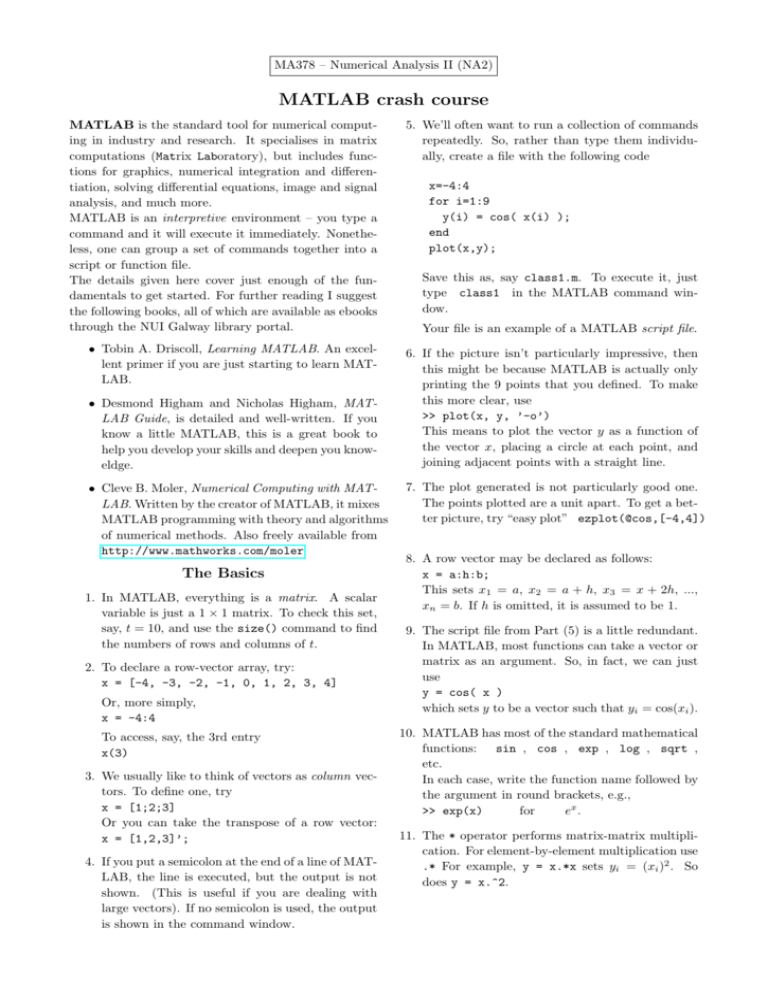
MA378 – Numerical Analysis II (NA2)
MATLAB crash course
MATLAB is the standard tool for numerical computing in industry and research. It specialises in matrix
computations (Matrix Laboratory), but includes functions for graphics, numerical integration and differentiation, solving differential equations, image and signal
analysis, and much more.
MATLAB is an interpretive environment – you type a
command and it will execute it immediately. Nonetheless, one can group a set of commands together into a
script or function file.
The details given here cover just enough of the fundamentals to get started. For further reading I suggest
the following books, all of which are available as ebooks
through the NUI Galway library portal.
5. We’ll often want to run a collection of commands
repeatedly. So, rather than type them individually, create a file with the following code
• Tobin A. Driscoll, Learning MATLAB. An excellent primer if you are just starting to learn MATLAB.
6. If the picture isn’t particularly impressive, then
this might be because MATLAB is actually only
printing the 9 points that you defined. To make
this more clear, use
>> plot(x, y, ’-o’)
This means to plot the vector y as a function of
the vector x, placing a circle at each point, and
joining adjacent points with a straight line.
• Desmond Higham and Nicholas Higham, MATLAB Guide, is detailed and well-written. If you
know a little MATLAB, this is a great book to
help you develop your skills and deepen you knoweldge.
• Cleve B. Moler, Numerical Computing with MATLAB. Written by the creator of MATLAB, it mixes
MATLAB programming with theory and algorithms
of numerical methods. Also freely available from
http://www.mathworks.com/moler
The Basics
1. In MATLAB, everything is a matrix. A scalar
variable is just a 1 × 1 matrix. To check this set,
say, t = 10, and use the size() command to find
the numbers of rows and columns of t.
2. To declare a row-vector array, try:
x = [-4, -3, -2, -1, 0, 1, 2, 3, 4]
Or, more simply,
x = -4:4
To access, say, the 3rd entry
x(3)
3. We usually like to think of vectors as column vectors. To define one, try
x = [1;2;3]
Or you can take the transpose of a row vector:
x = [1,2,3]’;
4. If you put a semicolon at the end of a line of MATLAB, the line is executed, but the output is not
shown. (This is useful if you are dealing with
large vectors). If no semicolon is used, the output
is shown in the command window.
x=-4:4
for i=1:9
y(i) = cos( x(i) );
end
plot(x,y);
Save this as, say class1.m. To execute it, just
type class1 in the MATLAB command window.
Your file is an example of a MATLAB script file.
7. The plot generated is not particularly good one.
The points plotted are a unit apart. To get a better picture, try “easy plot” ezplot(@cos,[-4,4])
8. A row vector may be declared as follows:
x = a:h:b;
This sets x1 = a, x2 = a + h, x3 = x + 2h, ...,
xn = b. If h is omitted, it is assumed to be 1.
9. The script file from Part (5) is a little redundant.
In MATLAB, most functions can take a vector or
matrix as an argument. So, in fact, we can just
use
y = cos( x )
which sets y to be a vector such that yi = cos(xi ).
10. MATLAB has most of the standard mathematical
functions: sin , cos , exp , log , sqrt ,
etc.
In each case, write the function name followed by
the argument in round brackets, e.g.,
>> exp(x)
for
ex .
11. The * operator performs matrix-matrix multiplication. For element-by-element multiplication use
.* For example, y = x.*x sets yi = (xi )2 . So
does y = x.^2.
MA378 – Numerical Analysis II (NA2)
Lab 1: Polynomial Interpolation
Goal: to investigate polynomial interpolation using some MATLAB routines.
In this class you will need to know the following.
Functions: You can define your own functions in MATLAB using a syntax such as
>> f = @(x)(exp(cos(x/2)))
Interpolation: >> polyfit(x,y,n) Returns the coefficients of the polynomial of degree n that interpolates
the pairs (xi , yi ). It returns a vector a where ai is the coefficient of xn−i .
Evaluating a polynomial:
the vector z.
>> polyval(a, z) evaluates the poly defined by the vector a at the points in
Plotting: >> plot(x,y,’o’) plots the points (xi , yi ) using circles.
>> plot(x,y,’o’, X, Y) plots the points (xi , yi ) (using circles) and the set (Xi , Yi ) on the same axes.
...............................................................................................................
Q1 Download lab1.m from Blackboard. Note how the function f is defined at the start.
This script computes p2 , the quadratic polynomial that interpolates f (x) = ecos(x/2) at the points x0 = −5,
x1 = 0 and x2 = 5. It also plots f (x) and p2 (x), along with the error : f (x) − pn (x), for −5 ≤ x ≤ 5.
Q2 Adapt this program to find p5 , the polynomial that interpolates f (x) = ecos(x/2) at 6 equally spaced points
between −5 and 5.
Q3 By experimentation, find n such that, if pn is the interpolant to f on n + 1 equally spaced points in [−5, 5],
then
kf − pn k∞ := max |f (x) − pn (x)| ≤ 10−6 .
−5≤x≤5
Q4 The above example, and the Weierstrass Approximation Theorem, might suggest that, for any function
f ∈ C n [a, b], if we take large enough n, we can find a polynomial that approximates f arbitrarily well.
However, this is not necessarily the case!
By changing the definition of the function f in your code, find p3 that interpolates Runge’s Function f (x) =
1/(1 + x2 ) on [−5, 5] at equally spaced points.
Now try for larger n in an effort to improve the accuracy of the approximation. Hence demonstrate that
lim kf (x) − pn (x)k∞ = ∞,
n→∞
for equally spaced interpolation nodes.
Q5 Instead of using equally spaced points, try choosing the points by hand. Start with x0 = −5, x1 = 0 and
x2 = 5. Now choose x3 and x4 in a way that you think will reduce the error. And then x5 and x6 and so on.
Using about 20 points you should be able to get the error close to 10−2 .
Tip: Since the function is symmetric about x = 0, just define, say, the points on [0, 5] and then extend to
[−5, 5] as follows: >> x = [0,3,5]; x = union(-x,x);
Or you can try using the ginput function that lets you pick points from a graph.
Q6 Although we won’t cover it in class, Chebyshev showed that, in general, one should choose points given by
the formula:
(i + 12 )π
b−a
b+a
xi =
cos
+
,
for i = 0, 1, . . . , n.
2
n+1
2
Try this for various n and test if it works. If you are interested, see p244 of the text for Mathematical details.
At the end of the lab, submit your answer for Q3, and your code for Q5 or Q6 (either will do) through the “Labs”
section of Blackboard.