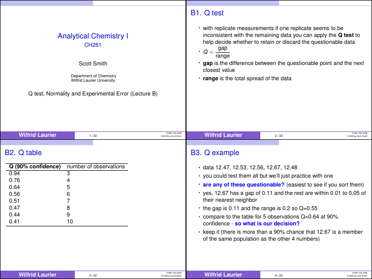
B1. Q test
• with replicate measurements if one replicate seems to be
Analytical Chemistry I
inconsistent with the remaining data you can apply the Q test to
help decide whether to retain or discard the questionable data
gap
• Q=
range
• gap is the difference between the questionable point and the next
closest value
CH261
Scott Smith
Department of Chemistry
Wilfrid Laurier University
• range is the total spread of the data
Q test, Normality and Experimental Error (Lecture B)
Wilfrid Laurier
1 / 22
CH261 Fall 2008
© 2008 by Scott Smith
B2. Q table
Q (90% confidence)
0.94
0.76
0.64
0.56
0.51
0.47
0.44
0.41
Wilfrid Laurier
2 / 22
CH261 Fall 2008
© 2008 by Scott Smith
B3. Q example
number of observations
3
4
5
6
7
8
9
10
• data 12.47, 12.53, 12.56, 12.67, 12.48
• you could test them all but we’ll just practice with one
• are any of these questionable? (easiest to see if you sort them)
• yes, 12.67 has a gap of 0.11 and the rest are within 0.01 to 0.05 of
their nearest neighbor
• the gap is 0.11 and the range is 0.2 so Q=0.55
• compare to the table for 5 observations Q=0.64 at 90%
confidence - so what is our decision?
• keep it (there is more than a 90% chance that 12.67 is a member
of the same population as the other 4 numbers)
Wilfrid Laurier
3 / 22
CH261 Fall 2008
© 2008 by Scott Smith
Wilfrid Laurier
4 / 22
CH261 Fall 2008
© 2008 by Scott Smith
B5. •Error
B4. Normality
• Normality is a concentration unit that takes reaction stoichiometry
into effect
• if reaction stoichiometry is 1:1 then normality is the same as
molality
• if you change the reaction the reagent (titrant) is used for its
normality changes
• for proton donation reactions, normality of 1 M HCl and 1 M
H2 SO4 ?
• for redox reactions normality is determined by the number of
electrons transfered
• normality is defined in appendix E of Harris.
Figure: There are errors associated with every measurement
Wilfrid Laurier
5 / 22
CH261 Fall 2008
© 2008 by Scott Smith
Wilfrid Laurier
6 / 22
CH261 Fall 2008
© 2008 by Scott Smith
B7. •Practice
B6. Significant Figures
• The number of significant figures is the minimum number of
digits needed to write a given value in scientific notation without
loss of accuracy
• leading zeros are not significant
• last digit (at least) has uncertainty
• some numbers have no uncertainty - can you think of an example?
• how many significant figures is 107400 ?
• try to estimate to the nearest tenth of a division
Figure: linear and logarithmic scales
Wilfrid Laurier
7 / 22
CH261 Fall 2008
© 2008 by Scott Smith
Wilfrid Laurier
8 / 22
CH261 Fall 2008
© 2008 by Scott Smith
B8. Sig Fig Arithmetic
B9. Rounding
• round on the final answer to avoid acculation of round-off errors
• example 1: 121.7943 = to 3 decimals
• (1) if the numbers being added or subtracted have equal number
• example 2: 43.55 = to 3 sig figs
of digits the answer goes to the same decimal place as the
individual numbers
• round to nearest even digit when last digit is a “5”
• example 3: 43.25 = to 3 sig figs
• this can lead to an increase or decrease in significant figures
• example 4: 43.2500001 = to 3 sig figs
• example 1: 5.345 + 6.728 =
• example 2: 7.26 × 1014 − 6.69 × 1014 =
• (2) if the numbers do not have equal numbers of digits the answer
is limited to the by the least certain one
• example 3: 18.9984032 + 18.9984032 + 83.798 =
Wilfrid Laurier
CH261 Fall 2008
9 / 22
© 2008 by Scott Smith
B10. Sig. Figs in × and ÷
digits contained in the number with the fewest significant figures
• example 1: (4.3179 ×
10 / 22
CH261 Fall 2008
© 2008 by Scott Smith
B11. Logarithms
• (3) in multiplication and division answer is limited to the number of
1012 )(3.6
Wilfrid Laurier
×
10−19 )
=answer
• power of 10 has no influence on the number of figures retained
• a logarithm is composed of a characteristic and a mantissa
• chacteristic is the integer part and the mantissa is the decimal part
• (4) the number of digits in the mantissa of a number should equal
the number of significant figures in that number
• example 1: characteristic and mantissa for log 339answer
• example 2: characteristic and mantissa for log(3.39e − 5)answer
• (5) the number of sig figs in the antilogarithm should equal the
number of digits in the mantissa
• example 3: 10−3.42 =answer
Wilfrid Laurier
11 / 22
CH261 Fall 2008
© 2008 by Scott Smith
Wilfrid Laurier
12 / 22
CH261 Fall 2008
© 2008 by Scott Smith
B12.• Sig fig graphing
B13. Sig fig graphing
Figure: showing trends
Wilfrid Laurier
13 / 22
Figure: meant to display quantitive behaviour
CH261 Fall 2008
© 2008 by Scott Smith
Wilfrid Laurier
14 / 22
CH261 Fall 2008
© 2008 by Scott Smith
B15.• Accuracy
B14. Systematic Error
• errors arising from flaw in the equipment or experimental design
are systematic errors
• these errors are reproducible and will lead to answers always too
high or too low (on or the other)
• can you think of some examples ?
• systematic errors can be indentifed and controlled
• random error may be positive or negative and cannot be removed
(but can possibly be minimized)
• can you think of some examples ?
• precision and accuracy are important concepts
Figure: before and after introduction of SRM
Wilfrid Laurier
15 / 22
CH261 Fall 2008
© 2008 by Scott Smith
Wilfrid Laurier
16 / 22
CH261 Fall 2008
© 2008 by Scott Smith
B16. Propagation of Uncertainty
B17. Propagation of Uncertainty
• for addition and subtraction the error is the square root of the
• for multiplication and division the error is the square root of
• for errors q
e1 , e2 and e3 for an arithmatic operation we can write
• for errors %e
q1 , %e2 and %e3 for a × or ÷ operation we can write
• example 1: (1.76 ± 0.03) + (1.89 ± 0.02) − (0.59 ± 0.02) =answer
(1.76 ± 0.03)(1.89 ± 0.02)
• example 1:
=answer
(0.59 ± 0.02)
the sum of squares of the absolute uncertainities
eoverall =
e12
+
e22
+
e32
• example 2: what is the percent relative uncertainty in example
the the sum of squares of the percent relative uncertainities
%eoverall =
%e12 + %e22 + %e32
1answer
Wilfrid Laurier
17 / 22
CH261 Fall 2008
© 2008 by Scott Smith
Wilfrid Laurier
18 / 22
CH261 Fall 2008
© 2008 by Scott Smith
B19.• Propagation of Uncertainty
B18. The Real Rule for Sig figs
• the first digit of the absolute uncertainty is the last significant
digit in the answer
(0.002364 ± 0.000003)
=answer
(0.02500 ± 0.00005)
• example 1:
Figure: Propagation of uncertainty rules
Wilfrid Laurier
19 / 22
CH261 Fall 2008
© 2008 by Scott Smith
Wilfrid Laurier
20 / 22
CH261 Fall 2008
© 2008 by Scott Smith
B20. Systematic Uncertainty
B21. Practice
• for systematic uncertainty arithmetic just add the uncertainties
• on tests I’ll give you table 3.1 (remind me!)
• this is because the uncertainties are not random
• the only good way to learn this stuff is practice and lots of it
• example 1: if a pipette delivers 25.00 ± 0.03 and you use it to
• all the problems in the chapter are good but the last few 3-19 to
deliver 100 mL, what is the uncertainty?
3-23 are a little trickier
• if the pipette is calibrated 24.991 ± 0.006 mL what is the
uncertainty ?
• 99.964 ± 0.012
Wilfrid Laurier
21 / 22
CH261 Fall 2008
© 2008 by Scott Smith
Wilfrid Laurier
22 / 22
CH261 Fall 2008
© 2008 by Scott Smith