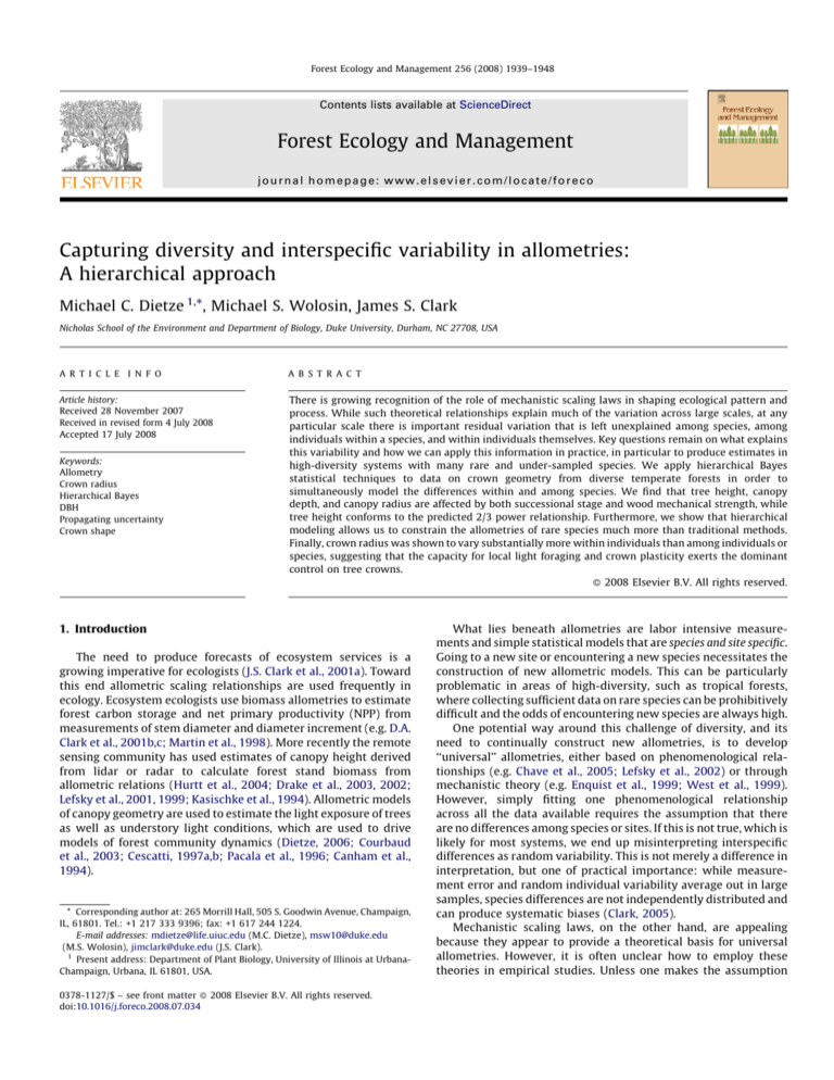
Forest Ecology and Management 256 (2008) 1939–1948
Contents lists available at ScienceDirect
Forest Ecology and Management
journal homepage: www.elsevier.com/locate/foreco
Capturing diversity and interspecific variability in allometries:
A hierarchical approach
Michael C. Dietze 1,*, Michael S. Wolosin, James S. Clark
Nicholas School of the Environment and Department of Biology, Duke University, Durham, NC 27708, USA
A R T I C L E I N F O
A B S T R A C T
Article history:
Received 28 November 2007
Received in revised form 4 July 2008
Accepted 17 July 2008
There is growing recognition of the role of mechanistic scaling laws in shaping ecological pattern and
process. While such theoretical relationships explain much of the variation across large scales, at any
particular scale there is important residual variation that is left unexplained among species, among
individuals within a species, and within individuals themselves. Key questions remain on what explains
this variability and how we can apply this information in practice, in particular to produce estimates in
high-diversity systems with many rare and under-sampled species. We apply hierarchical Bayes
statistical techniques to data on crown geometry from diverse temperate forests in order to
simultaneously model the differences within and among species. We find that tree height, canopy
depth, and canopy radius are affected by both successional stage and wood mechanical strength, while
tree height conforms to the predicted 2/3 power relationship. Furthermore, we show that hierarchical
modeling allows us to constrain the allometries of rare species much more than traditional methods.
Finally, crown radius was shown to vary substantially more within individuals than among individuals or
species, suggesting that the capacity for local light foraging and crown plasticity exerts the dominant
control on tree crowns.
ß 2008 Elsevier B.V. All rights reserved.
Keywords:
Allometry
Crown radius
Hierarchical Bayes
DBH
Propagating uncertainty
Crown shape
1. Introduction
The need to produce forecasts of ecosystem services is a
growing imperative for ecologists (J.S. Clark et al., 2001a). Toward
this end allometric scaling relationships are used frequently in
ecology. Ecosystem ecologists use biomass allometries to estimate
forest carbon storage and net primary productivity (NPP) from
measurements of stem diameter and diameter increment (e.g. D.A.
Clark et al., 2001b,c; Martin et al., 1998). More recently the remote
sensing community has used estimates of canopy height derived
from lidar or radar to calculate forest stand biomass from
allometric relations (Hurtt et al., 2004; Drake et al., 2003, 2002;
Lefsky et al., 2001, 1999; Kasischke et al., 1994). Allometric models
of canopy geometry are used to estimate the light exposure of trees
as well as understory light conditions, which are used to drive
models of forest community dynamics (Dietze, 2006; Courbaud
et al., 2003; Cescatti, 1997a,b; Pacala et al., 1996; Canham et al.,
1994).
* Corresponding author at: 265 Morrill Hall, 505 S. Goodwin Avenue, Champaign,
IL, 61801. Tel.: +1 217 333 9396; fax: +1 617 244 1224.
E-mail addresses: mdietze@life.uiuc.edu (M.C. Dietze), msw10@duke.edu
(M.S. Wolosin), jimclark@duke.edu (J.S. Clark).
1
Present address: Department of Plant Biology, University of Illinois at UrbanaChampaign, Urbana, IL 61801, USA.
0378-1127/$ – see front matter ß 2008 Elsevier B.V. All rights reserved.
doi:10.1016/j.foreco.2008.07.034
What lies beneath allometries are labor intensive measurements and simple statistical models that are species and site specific.
Going to a new site or encountering a new species necessitates the
construction of new allometric models. This can be particularly
problematic in areas of high-diversity, such as tropical forests,
where collecting sufficient data on rare species can be prohibitively
difficult and the odds of encountering new species are always high.
One potential way around this challenge of diversity, and its
need to continually construct new allometries, is to develop
‘‘universal’’ allometries, either based on phenomenological relationships (e.g. Chave et al., 2005; Lefsky et al., 2002) or through
mechanistic theory (e.g. Enquist et al., 1999; West et al., 1999).
However, simply fitting one phenomenological relationship
across all the data available requires the assumption that there
are no differences among species or sites. If this is not true, which is
likely for most systems, we end up misinterpreting interspecific
differences as random variability. This is not merely a difference in
interpretation, but one of practical importance: while measurement error and random individual variability average out in large
samples, species differences are not independently distributed and
can produce systematic biases (Clark, 2005).
Mechanistic scaling laws, on the other hand, are appealing
because they appear to provide a theoretical basis for universal
allometries. However, it is often unclear how to employ these
theories in empirical studies. Unless one makes the assumption
1940
M.C. Dietze et al. / Forest Ecology and Management 256 (2008) 1939–1948
that the slope and intercept predicted by a theoretical model are
exactly correct, there is no clear way in classical statistics to
combine this information with empirical data. Mechanistic
relationships are also usually verified with data sets that span
many orders of magnitude; while on a large scale species are more
alike than different, at any particular scale there may be a large
amount of unexplained variation. Indeed, one of the short comings
of the search for universal allometries is that most research has
given less attention to explaining why species are different and
what factors, whether they be driven by life-history, mechanical
limits, or phylogenetic constraint, predict the variation among
species; research that accounts for the variability among species
and sites in scaling is still in early development (e.g. Enquist et al.,
2007; Price et al., 2007). While not directly applicable to empirical
studies themselves, these theories do have the potential to increase
the efficiency of developing relationships for new species and sites
if they can be combined effectively with data.
Fortunately, modern statistical methods provide an alternative,
Bayesian hierarchical models, that can accommodate the challenges of diversity—the theoretical need to account for inter- and
intraspecific variation and the empirical need to make predictions
for rare species. Essentially, hierarchical models enable us to fit one
relationship for each species, just as the species-specific approach
would, while simultaneously fitting a ‘‘universal’’ relationship
across species that constrains the species-specific relationships.
How much constraint to provide is determined automatically by
the data. If species are similar, the across-species relationship
provides stronger constraint, which then strengthens the fit of rare
species where data are limited. The hierarchical model can even be
used to predict the sampling distribution of allometric relationships for unobserved species. While measuring new species
directly is always preferable, extrapolation across species is often
necessary, especially in hyperdiverse regions, and the hierarchical
modeling framework provides both constraints on this extrapolation and an estimate of the uncertainty this introduces, rather than
simply applying equations developed for other species as if this
introduced no additional error. Essentially, Bayesian hierarchical
models provide an intermediate between the two extremes
(species-specific vs. universal allometries) that preserves the
strengths of both approaches while reducing both their limitations.
The hierarchical approach achieves this because it acknowledges
that the growth forms of trees are generally similar across species,
but that they are not the same.
In addition to handling rare and novel species, there are a
number of aspects of the Bayesian hierarchical framework that
allow us to make greater use of the data and improve our
ecological understanding: the incorporation of information
from mechanistic scaling laws, the dependence of interspecific
variability on life-history, biomechanics, and phylogenetic constraint, and the ability to model missing or indirectly observed
data. In Bayesian hierarchical models the constraints provided by
mechanistic scaling theory enter seamlessly as a prior on the
across-species allometry. Similarly, we can explore the effects of
species-level differences, such as differences in life-history,
mechanics, or phylogeny, by including these as covariates in
the across-species model. This is the same idea that underlies the
current interest in tying biomass allometries to wood density (e.g.
Chave et al., 2005), but in a more rigorous framework. Finally, the
quantities of interest are not always directly observed or
observable. For example, we infer the shape and structure of
tree canopies based on proxies such as ground measurements of
crown extent or LIDAR profiles. Hierarchical Bayesian methods
provide a straightforward means of estimating such ‘‘latent’’
variables by decomposing a complex problem into simple
conditional probabilities that can be sampled over, defining the
statistical relationship between the observed and unobserved
quantities. In a similar way Bayesian methods can sample over
the distributions of missing data, reducing the necessity of
throwing out useful information because of the occasional
missing measurement or covariate. Most importantly, these
approaches can lead to a greater ecological understanding of the
underlying processes. For example, below we model canopy
radius as a latent variable and are thus able to partition residual
variability to within-crown and between-crown components.
This analysis points to the dominant role of individual-level
dynamics, such as crown light foraging, rather than sizedependant scaling, in controlling crown shape and size, but
would have been impossible if we had simply worked with
sample-mean canopy radius.
For the goal of ecological forecasting, perhaps the greatest
strength of the hierarchical Bayes framework is that it provides a
unified rigorous framework for inference and prediction. Current
allometric models are often applied assuming the parameters with
the highest likelihood are ‘‘true’’ and ignoring uncertainty. However,
the propagation of uncertainty through forecasts is critical to
assessing their accuracy and their usefulness to managers and policy
makers; ignoring uncertainty leads to overconfident prediction.
Forecasting in a Bayesian framework is no more complicated than
sampling over the posterior parameter and error distributions to
generate predictive distributions. Propagating this error through
further analyses is as simple as sampling from the predictive
distributions and performing whatever calculations are needed,
whether it be a simple summation of stand biomass or a complex
nonlinear simulation model.
In this paper we present an analysis of an allometric model of
tree height and crown geometry using a hierarchical Bayes
approach. This model is a complex multivariate analysis with
species-level covariates that estimates allometric relationships
while addressing a wide range of issues encountered with real
data. The model is fit to field measurements made in the Carolina
Piedmont and the Southern Appalachians. Below we outline the
field methods used and derive our statistical models step by step,
addressing specific issues and explaining how we improve upon
previous approaches. The West, Brown, and Enquist (WBE)
metabolic scaling theory is incorporated as a moderately
informative prior to constrain the across-species scaling of tree
height (West et al., 1999; Enquist et al., 1999). This analysis shows
that hierarchical Bayes methods can provide biologically more
reasonable estimates for rare species or species with a narrow
observed size range. Furthermore, we find that shade tolerance and
wood mechanical strength affect canopy geometry, with shadetolerant species producing thick trunks with wide and deep
canopies. Canopy depth also increases with wood strength. Overall,
we find that the tree height allometry is consistent with the
predicted 2/3 scaling law across a wide range of priors, but that
canopy radius departs considerably from the predicted 2/3 scaling
(West et al., 1999; Enquist et al., 1999). Canopy radius is shown to
have greater variability within individuals than among, highlighting the importance of individual-level dynamics such as light
foraging by tree crowns.
2. Methods
2.1. Field methods
Total tree height, height to base of crown, and crown radius
were measured with a laser range finder (Impulse 2000, Lasers
Technology Inc., Englewood, Colorado) for a subset of trees from
two mapped stands in the southeastern US. The first stand
(4.3 ha) is located in the Blackwood Division of Duke Forest, in
M.C. Dietze et al. / Forest Ecology and Management 256 (2008) 1939–1948
Chapel Hill, NC (358590 N latitude, 798060 W longitude) in the
Carolina Piedmont. Half of the stand is oak-hickory forest, while
the other half is 80-year-old loblolly pine (Pinus taeda) with
significant hardwood ingrowth. The second stand (4.8 ha) is
located at the Coweeta LTER site in Otto, NC (358030 N latitude,
838270 W longitude) in mixed hardwood forest. Detailed site
descriptions can be found at http://www.env.duke.edu/forest and
http://coweeta.ecology.uga.edu for Duke Forest and Coweeta
respectively while detailed stand information is in Dietze
(2006). In 2000 all trees over 2 m tall were identified, mapped,
and measured for diameter at breast height (DBH). For some taxa
proper identification to species was difficult and individuals were
recorded at the genus level. All unidentified Quercus were among
the red oaks (Quercus section Lobatae), which are particularly
prone to hybridization making species-level identification occasionally difficult. Taxonomy follows Radford et al. (1968) with the
exceptions of Quercus montana (chestnut oak, was Quercus prinus)
and Frangula caroliniana (Carolina buckthorn, was Rhamnus
caroliniana).
Crown geometry data are drawn from two sampling efforts for a
combined sample size of 1691 trees measured for 53 species. In the
first sample (2001 data), designed specifically to estimate
allometries, trees were selected from the stand database in a
stratified random manner to insure maximal coverage of all species
and sizes. For each tree we measured DBH, height, height to base of
crown, and maximum and minimum crown radius. The base of the
crown was taken to be the lowest foliage on the lowest major
branch and thus excluded young epicormic branches. The second
sampling effort (2003 and 2004) was collected to compare canopy
measurements made on the ground to those from aerial
videography (Wolosin, 2007) and consists of tree height, height
to base of crown, and canopy radius in the eight cardinal compass
directions. Heights and radii were measured using a laser range
finder (Impulse 2000, Lasers Technology Inc., Englewood, Colorado) with a build-in digital clinometer that was custom modified
with a mirrored vertical sight to enable accurate identification of
the crown edge. Since crown radii are measured as vectors from the
trunk, it is possible for radii to have negative values for irregularly
shaped crowns.
The species-level covariates that we consider in the crown
geometry model include phylum, shade tolerance, and wood
strength. Shade-tolerance classification is based on estimates
from the U.S. Forest Service (USFS) Silvics Manual (Burns and
Honkala, 1990) and the USFS Fire Effects Information System
(FEIS) database (http://www.fs.fed.us/database/feis/), both of
which rely heavily on Baker (1948). The shade-tolerance classes
were converted into an ordinal ranking (very tolerant = 1, very
intolerant = 5). Mechanical properties were taken from the USFS
Forest Products Lab database (http://www2.fpl.fs.fed.us/) and
Wood Handbook (Forest Products Laboratory 1999). For this
analysis we use the compressive strength of green wood parallel
to the grain (kPa), which is more likely to be directly related to
overall tree strength than more common surrogates such as wood
density (Woodcock, 2003; Chave et al., 2005). In this analysis
phylum enters as a gymnosperm/angiosperm indicator variable,
though more sophisticated approaches using greater taxonomic
resolution or phylogenetic distance could easily be developed. The
complete list of species, covariates, and sample sizes is given in
Table S1.
2.2. Bayesian hierarchical allometries
In this section we describe the Hierarchical Bayes model we use
to fit crown allometries. We begin by explaining the simplest
possible allometric model and then progress through the steps of
1941
model specification, explaining what each new part does, until we
reach the full model. The allometric model that serves as the base
of our analysis is the traditional power–law relationship,
y ¼ b0 xb1 ;
which is commonly used to assess scaling rules in many scientific
disciplines. Power–law relationships produce a strait line on a
log–log graph and are usually fit by either Ordinary Least Squares
(OLS) or Reduced Major Axis (RMA) linear regression Yij = Xijbj
+ eij where Yij = log(yij), Xij = {1,log(xij)}, bj = {log(b0),b1,j}, and
ei j Nð0; s 2j Þ is normally distributed residual error. Throughout
this manuscript we use subscripts i and j to denote individual and
species, respectively; here the j subscripts denote that each
species is being fit separately. A complete Bayesian specification
requires that we provide prior distributions on the parameters bj
and s. The prior on bj is normal, bj N(Bj, Fj), where Bj and Fj are
the prior mean and variance. An inverse-gamma distribution,
s2 Inverse Gamma(a,g), is the standard choice of prior on the
variance because of its conjugacy and because the parameters a
and g are interpretable as the prior contribution to the sample
size and sum-of-squares respectively. Finally, we assume that
measurement error in our x variable, tree diameter, is negligible
compared to error in the crown measurement, though incorporating this error is straightforward in the Bayesian framework.
Fitting each species separately ignores the fact that the growth
forms of trees are generally similar across species. An alternative to
this is to treat all individuals as being drawn from one universal
allometry, Yi N(Xib,s2), that drops species effects (subscript j).
These two cases form the bounding extremes: all species are
different vs. all species are the same. The intermediate approach is
to model each species’ parameters as being drawn from a common
pool:
b j NðB; FÞ
(1)
where B is the across-species universal allometry from which
species-specific allometric coefficients, bj, are drawn and F is the
‘‘global’’ covariance matrix. If the global allometric parameters (B,
F) are set to fixed values determined a priori, Eq. (1) is the same as
the by-species approach above but with all species having the
same prior.
It is through the use of priors that we formally include the
predictions of mechanistic scaling models into our statistical
analysis. However, this method only allows the prior, not the data,
to inform the universal allometry. We can improve upon this by
allowing B and F to be fit parameters, making this a hierarchical
Bayes model. When we do this we need to construct hyperpriors on
B and F rather than priors on bj; to do this we use the mechanistic
prior to be the constraint on the across-species allometric model:
B NðB0 ; V 0 Þ
F Inv Wishartðw; wC Þ
;
(2)
where the inverse-Wishart distribution in the multivariate
generalization of the inverse-gamma described earlier. This
approach allows the universal allometry to be informed both by
data and prior information. The degree to which the allometric
relationships are similar across species controls the variance in B
and F and thus the strength of the hierarchical universal allometry
in constraining the species-level fits. Rare species are constrained
by the hierarchical structure to be ‘‘tree like,’’ while for common
species the data will dominate the fit unless the hierarchical
constraint is very strong. The hierarchical structure also allows us
to formally define the predictive distribution for unobserved
species.
1942
M.C. Dietze et al. / Forest Ecology and Management 256 (2008) 1939–1948
2.3. Canopy geometry model
Field-measured tree crowns are defined by three measurements: tree height, height to base of canopy, and canopy radius.
We therefore expand the basic allometric model to the multivariate case
Y i j NðX i j b j ; SÞ
T
Y i j ¼ ½Hi j ; ui j ; Ri j X i j ¼ ½1; Di j T
(3)
where H = log(tree height), u = logit(relative canopy depth),
R = log(canopy radius), D = log(DBH), S is a 3x3 covariance matrix,
and relative canopy depth is defined as 1-(height to base of crown)/
(tree height). The decision to fit all three-response variables
simultaneously using a full covariance matrix, rather than to fit
each variable separately, acknowledges the fact that response
variables are likely related to each other. The use of logit
transformed relative canopy depth, rather than a direct power–
law fit to canopy depth, is a simple way to constrain the bottom of
the canopy to be between the top of the tree and the ground at all
diameters. The alternative of fitting a power–law to the canopy
base height requires constraining the slope to be the same as that
of total tree height, meaning that relative canopy depth is always
constant for a given species. The logit transform of relative canopy
allows canopy depth to vary with tree size and allows us to easily
incorporate the transformed values in a regression framework.
To include species-level covariates we simply modify Eq. (1) to
b j NðZB; FÞ
(4)
where Z is the matrix of species-level covariates. By including
species-level covariates at this higher level of the hierarchical
model, we are formally including these variables in the model in a
way that includes the uncertainty we have in the bj’s when trying
to explain patterns among species. This is in contrast with post-hoc
methods which treat the bj’s as fixed and regress them against the
species-level covariates. Such an approach is not only overconfident in its predictions, since it fails to propagate uncertainty
in the regression parameters, but also falsely treats each species as
representing the same amount of information. Furthermore, by
modeling the process in a hierarchical manner with covariates, we
are able to reduce the uncertainty we have in predictions of rare
and unobserved species when we know their covariates.
An added complication for this model is that we do not observe
canopy radius directly, but rather observe 2–8 samples of the
canopy radius from which we infer radius. Rather than average
these samples beforehand, and thus discard the large withinindividual variability in canopy radius, we formally incorporate it.
If we let Ri be a latent variable for the ‘‘unobserved true’’ canopy
radius of individual i and DBHi s 2R be the size-dependent withinindividual variance in canopy radius, then we model canopy radius
as
r i;k Nðri ; DBHi s 2R Þ;
where ri,k is the kth radius measurement of individual i. r* can be
thought of as either the average canopy radius or the radius of a
circular crown with area equivalent to the crown area, both
definitions being equivalent in the limit. The linear scaling of the
radius variance with diameter was done in order to make the
residuals homoskedastic after exploratory analyses revealed
unsurprisingly that large trees had greater within-crown variability in radius. A single sR was used for the two sampling
campaigns because initial analyses suggested they had similar
variance, though fitting variances separately for each data set is
straightforward in this framework.
The Bayesian framework allows us to formally account for
the fact that we are missing species-level covariates, Zmis, for
some species (Table S1). We assume the missing data to be
missing at random and that the missing-data mechanism is
ignorable, in the formal sense that parameters controlling the
allometries and those controlling the missing-data imputation
are independent in the prior distribution. For simplicity we treat
the Z variables as having a multivariate normal distribution,
p(ZjmZ,sZ) N(mZ,sZ), from which Zmis can be drawn. When one
or more of the covariates is known, the remaining can be drawn
from the appropriate marginal distribution conditioned on the
known values.
To fully specify the model in a Bayesian context we make use
of standard conjugate priors wherever possible. The model was
fit making use of standard MCMC methods (Clark, 2007; Gelman
et al., 1995). For most of the parameters we are able to use a
Gibbs sampler to sample directly from the conditional distributions. In order to incorporate existing predictions into the
across-species allometry prior (B0, Eq. (2)), we used the slope
predicted from WBE (West et al., 1999; Enquist et al., 1999) for
tree height (2/3) and set the intercept to 1/4 in order to produce
reasonable heights. Logit crown depth priors were set to have 0
slope and a 0 intercept (which gives a crown depth of 50%
irrespective of DBH) based on the fixed crown depths in Pacala
et al. (1996). Crown radius priors were set at a slope of 1/2,
based on the assumption that crown area would scale linearly,
and an intercept of 0.3 to produce reasonable radii. The prior
variance (V0) was set to a moderately informative but not strong
value (10). The remaining priors and conditional sampling
distributions are provided in the appendix. Model fitting was
done on a Linux workstation using R 2.1.1 (R Development Core
Team, 2005).
To determine the importance of the species-level covariates
we compared models using predictive loss with a squared error
loss function (Gelfand and Ghosh, 1998). Predictive loss was
chosen over other model selection criteria, such as DIC or Bayes
factors, primarily because of its emphasis on predictive
distributions since allometries are most often used for predictive
purposes. The predictive loss metric, D, aims to balance model
residual sum-of-squares error (G), which tends to decrease with
model complexity, and model predictive variance (P), which
tends to increase with model complexity due to high parameter
uncertainty, by selecting the model which minimizes their sum,
D = G + P. For the purpose of calculating predictive loss, as well as
all other posterior means, moments, and credible intervals, we
discarded the initial 20% of the MCMC to reduce burn-in effects
and 50% of the remaining sample to reduce autocorrelation.
Model selection was based on 30,000 MCMC steps, and then the
best fitting model was run for a total of 50,000 MCMC steps.
Initially, five versions of the model were compared: the full
hierarchical model with all covariates (FULL), the hierarchical
model without any covariates (INT), the FULL and INT models
with the universal variance T being drawn from inverse-Gamma
distributions rather than the joint inverse-Wishart (IG FULL, IG
INT), and a non-hierarchical implementation where each species
is fit independently (BYSPP). The IG models, which only estimate
the diagonal of the covariance matrix T, were added after initial
runs suggested that there may not be enough information at the
hierarchical level (53 species) to constrain the full covariance
matrix (21 parameters in the full model versus 6 in the IG). This
was supported by model selection which ranked the IG INT and
IG FULL models first and second respectively. Following this we
ran the IG model for all permutations of species-level covariates
in order to select the most parsimonious parameters, again using
predictive loss.
M.C. Dietze et al. / Forest Ecology and Management 256 (2008) 1939–1948
3. Results
Model selection showed that the model with inverse-gamma
variance and shade-tolerance class and mechanical strength as
hierarchical covariates had the lowest predictive loss (Table S2).
Models with inverse-gamma hierarchical variance (i.e. diagonal
variance structure) were supported over those with an inverseWishart variance (i.e. full covariance matrix), suggesting that the
full matrix was overfitting the data and that there was insufficient
information in 53 species to identify all 15 terms in the 6x6 matrix.
Overall, model selection suggested that there were no significant
differences in crown allometry between angiosperms and gymnosperms once shade tolerance and wood strength were included
and that there was little covariance across species in the three
measures of crown shape (tree height, crown depth, and crown
radius).
3.1. Species relationships
Looking at the species-level, Fig. 1 shows examples of the log–
log fit of the tree height–diameter relationship with 95% credible
intervals in comparison to the traditional linear regression fit. It is
immediately apparent that for species with a large sample size, and
where samples are well distributed across sizes, the two methods
of analysis produced essentially the same fit (Fig. 1 left column).
This is to be expected because the species data appropriately
overwhelm the hierarchical prior. However, for rare or poorly
distributed species the hierarchical model and linear regression
1943
can differ considerably. In these cases the ability of the hierarchical
model to borrow strength across species produced much more
biologically realistic relationships. For example, only large
individuals of black walnut (Juglans nigra, JUni), unclassified red
oaks (QUun), and Virginia pine (Pinus virginiana, PIvi) were found
in the study area and the classical regression model produced a
spurious negative correlation between diameter and height for the
first two and too shallow a slope for the third (Fig. 1 center
column). Similarly for rare understory tree species (Frangula
caroliniana, FRca, Halesia carolina, HAca, and Viburnum rufidulum,
VIru), the classical regression fits were either considerably too flat
or too steep (Fig. 1 right column). While the sample sizes for the
rare species in this study are small, they often represent a complete
census of the available stems and the sample sizes found here are
for the most part not uncommon in the literature. Thus, while the
poor frequentist fits may appear a bit of a strawman, they do
represent the only option available in the classical framework
other than arbitrarily applying the allometry of a different species.
Plots of height, canopy depth, and canopy radius for an example
species (Quercus rubra) are in Fig. 2 while plots for all species are in
Figs. S1–S4 and posterior mean parameter estimates are given in
Table S3.
The error covariance matrix (S) suggests that there was a positive
correlation in the residuals between log tree height and logit canopy
depth, such that trees that were taller than average for their
diameter also had deeper canopies (Table 1). The residuals of canopy
radius, on the other hand, were not correlated with tree height or
canopy depth. There was little residual variance in canopy height
Fig. 1. Height versus diameter log–log allometry model fits for example species. Posterior median model fit is depicted in the solid black lines while the posterior credible
intervals (95%) are shown in grey lines. Data are given in open black circles while the frequentist linear regression fit is given by a red line. Horizontal blue lines indicate the
‘‘mature height’’ of each species as reported in the USDA Plants Database (http://plants.usda.gov). For species with adequate data the Hierarchical Bayes model and the linear
regression model are very similar (acru = Acer rubrum, nysy = Nyssa sylvatica, ulal = Ulmus alata), while for species with limited data, and/or with data for only small
(frca = Frangula carolina, haca = Halesia carolina, viru = Viburnum rudifolium) or large trees (juni = Juglans nigra, quun = Quercus section Lobatae, pivi = Pinus virginiana), the
hierarchical fit constrains these species to more biologically realistic portions of the parameter space. All panels are on the same scale and have log10 diameter breast height
on the x-axis (1–100 cm) and log10 total tree height (meters) on the y-axis.
M.C. Dietze et al. / Forest Ecology and Management 256 (2008) 1939–1948
1944
Fig. 3. Within individual (solid line) and among individual (dashed line) variability
in tree canopy radius as a function of DBH.
3.2. Canopy radius
Fig. 2. Canopy allometry of red oak (Quercus rubra). The fits of total tree height (m),
relative canopy depth, and canopy radius (m) versus diameter. The solid red dots
show the observed data for tree height and canopy depth and the posterior means of
the ‘‘true’’ canopy radius latent variable for canopy radius, while the smaller blue
dots show all the radius measurements. A small portion of observed radii are less
than 0 m or greater than 10 m. (For interpretation of the references to color in this
figure legend, the reader is referred to the web version of the article.)
(0.0095), with the allometric model explaining 93% of the height
variance in the log scale and 85% in the linear scale. By comparison,
the canopy depth model had higher variance (0.57). However, on a
linear scale this model still explains 81% of the variance in canopy
depth. The variance in canopy radius is more complicated to assess
because it was treated as a latent variable.
Fig. 2 (bottom) shows both the raw canopy radius data (blue)
and the posterior means of the canopy radius latent variables (red).
These plots show a large amount of variability in the individual
measurements of canopy radius compared to the variability in the
latent mean radius. The method of treating canopy radius as a
latent variable not only allowed us to propagate uncertainty in the
canopy radius, which was informed by the samples of each tree’s
radius, but it also allowed us to partition the variance in canopy
radius. Fig. 3 shows that there was clearly more variance in canopy
radius within individual trees than among trees. It should be noted
that this is not obvious a priori. If the crowns of individual trees
were generally round but varied a lot in average radius, for
example, due to local neighborhood effects, the overall variability
in crown radius would be high (as are the blue points in Fig. 2) and
would have to be higher than the overall variability in mean radius
(red points), but the variability within trees would be low and the
variability among trees would be high.
3.3. Across-species model
The hierarchical across-species parameter posterior means and
variances of the best fitting model are reported in Table 2 along
with their 95% credible intervals. Overall, the effects of shade
tolerance tended to be stronger than the effects of mechanical
strength (Fig. 4). Shade intolerant trees were taller for a given
diameter, which was largely a result of intolerant trees having a
larger intercept rather than a different scaling exponent. In terms
of canopy depth, shade-tolerant trees had both deeper canopies
than shade intolerant trees (larger intercept) and got deeper at a
faster rate (larger slope). Shade-tolerant trees also had a larger
Table 1
Allometry species-level error covariance matrix (S)
Height
Depth
Radius
Height
Depth
Radius
0.0095 (0.0088, 0.0101)
0.011 (0.0075, 0.0153)
0.57 (0.53, 0.61)
1.5e5 (2.4e4, 2.8e4)
1.6e4 (1.8e3, 2.2e3)
0.0018 (0.0013, 0.0025))
Values are reported as posterior means and 95% posterior credible intervals. The off diagonal covariance elements show that residual variability in canopy geometry is not
correlated.
M.C. Dietze et al. / Forest Ecology and Management 256 (2008) 1939–1948
1945
Table 2
Species-level effects
Height intercept
Height slope
Depth intercept
Depth slope
Radius intercept
Radius slope
Intercept
Shade tolerance
Wood Strength
Variance
0.32 (0.08, 0.56)
0.59 (0.33, 0.85)
0.31 (0.07, 0.59)
0.33 (0.10, 0.60)
0.03 (0.26, 0.22)
0.37 (0.12, 0.63)
0.03 (0.02, 0.08)
0.00 (0.06, 0.05)
0.05 (0.10, 0.00)
0.05 (0.11, 0.00)
0.04 (0.09, 0.01)
0.01 (0.04, 0.06)
0.02 (0.22,0.16)
0.01 (0.18,0.23)
0.09 (0.31,0.09)
0.03 (0.23,0.15)
0.03 (0.16,0.24)
0.01 (0.22,0.19)
0.054
0.052
0.023
0.026
0.044
0.054
(0.033,0.082)
(0.032,0.080)
(0.015,0.034)
(0.017,0.039)
(0.028,0.068)
(0.033,0.085)
Parameters values (B & T in Eq. (4)) are reported with 95% credible intervals given in parentheses. Shade tolerance varies from 1 (very tolerant) to 5 (very intolerant) while
wood strength (bending moment) has been normalized by the mean (23900 kPa). The variance term represents the residual variance among species in their slope and
intercept parameters (b).
canopy radius, but as with height the difference was more
influenced by a difference in intercept than in scaling exponent. In
terms of mechanical strength the only discernable effect was on
crown depth intercept, such that species with stronger wood had
deeper canopies.
4. Discussion
The hierarchical Bayes model performed well at estimating the
allometric relationships for the fifty-three species in the study
area. While the height and canopy radius show clear agreement
between the data and models, the relative canopy depth allometry
was much noisier, suggesting that size is not the strongest
constraint on this variable. This is not too surprising since the
model did not take into account the local neighborhood
conditions, which should affect self-pruning. One area for further
model refinement would be the incorporation of stand and
neighborhood covariates, such as stem density, basal area, or site
factor. Adding additional species-level covariates is straightforward in the current modeling framework. Additional acrossspecies covariates, such as growth form and maximum tree
height, could easily be explored in this approach and would be
particularly beneficial for constraining rare shrubs and understory trees, though if the aim is to understand across-species
variation rather than just prediction care must be taken to avoid
circularity. In particular, due to the inherent unreliability of
extreme value statistics, data on maximum tree height, diameter,
and crown size would more appropriately enter as an additional
data source rather than as a covariate.
The estimation of canopy radius using a latent variable approach provided novel estimates of canopy radius that accounted for
both within and among crown variability and propagated the
uncertainty in mean radius into the allometric model in a clear and
defensible manner. The fact that within canopy variability is
greater than variability among canopies suggests that future work
focus on explaining within-individual crown dynamics. Indeed, a
more detailed analysis of high-resolution remote imagery from
these stands finds that modeling individual-level crown movement and light foraging is critical for predicting both the
ground and canopy-level light environment and adult growth
rates (Wolosin, 2007). Interestingly, this analysis finds similar
life-history and mechanical constraints on foraging as we do on
allometries.
Almost all allometric relationships are faced with the general
challenge of describing a snapshot of form and from this trying
to infer a process of growth that is plastic and the result of an
unknown individual history. This was a clear problem for estimating
canopy depth and radius, which show significant variability around
simple power–law relationships. The most obvious solution to
this is to follow and model the process of growth itself. While
estimates of tree diameter growth are commonplace, and measurements of height growth are not uncommon, measurements of
canopy growth are much more rare (Clark et al., 2004). However,
growth information would allow a much greater understanding of
canopy dynamics than just increasing the sample size of canopy
allometric models or further increasing the complexity of the
current analysis. Indeed, much of the ‘‘noise’’ in the allometries
represents true individual-level variability, rather than measurement error or model mismatch. Using such growth data, Bayesian
hierarchical models provide a clear and formal method for
separating individual effects from measurement error (Clark
et al., 2003, 2004).
At the hierarchical across species-level, the model provides a
balance between species-specific and universal allometries. For
rare species, and species with a limited size range, the hierarchical
model is a great improvement over conventional approaches. This
analysis successfully demonstrates the ability of this method to
deal with the diversity of the southeast US, an area that has high
woody plant diversity for the temperate region, and shows that the
model has high potential for application in hyperdiverse regions,
such as tropical rain forests.
The effects of the across-species covariates were generally
intuitive and consistent with the literature (Aiba and Kohyama,
1997; Ackerly and Donoghue, 1998; Kohyama et al., 2003; Poorter
et al., 2006; Sterck et al., 2001)—shade-tolerant species are
generally shorter with broad and deep crowns. These patterns are
consistent across many ecosystems and are generally interpreted
from the perspective of successional trade-offs between fast
vertical growth of slender stems and crowns, which potentially
risk higher self-shading, decreased mechanical stability, and
higher respiration and mortality in order to reach the canopy as
quickly as possible versus slow growing, broad and deep crowned
species with low mortality in low-light conditions (King, 1990;
Aiba and Kohyama, 1997; Kohyama et al., 2003). What is novel in
this analysis is that we found that there was greater variability in
allometric intercepts than in their slopes. This result is consistent
with mechanistic scaling laws, such as the West, Brown, and
Enquist (WBE) metabolic theory (West et al., 1999), which suggest
that there are basic physiological constraints on scaling exponents. To our knowledge, the various extensions to the WBE
theory have not made specific predictions about how these largely
hydraulic constraints should interact with the energetic considerations and demographic trade-offs along the successional
gradient. The additional effects of wood strength are also
interesting in that they suggest that there is residual variation
to explain beyond both the primarily hydraulic argument
presented in WBE’s theory and the successional gradient of
shade-tolerance.
Unfortunately, these hierarchical covariate effects were generally weak. Part of the reason for weak effects is that we are
propagating the uncertainty in the species-level allometric
parameters into the fitting of the across-species model, and thus
our results reflect this additional uncertainty and do not create a
false precision that would come from fitting to parameter means.
1946
M.C. Dietze et al. / Forest Ecology and Management 256 (2008) 1939–1948
Fig. 4. Effects of species-level covariates on the variation across species in crown allometries. For shade tolerance, curves go from very tolerant (blue) to very intolerant (red), while
for wood strength they go from 50% of the mean strength (blue) to 150% (red), which is approximately the range of variability observed. Shade intolerant species tend to be taller for
a given diameter, while tolerant species tend to have both deeper and wider crowns. In comparison, the effects of wood strength were much weaker, but suggest that stronger trees
tend to be taller and have wider but shallower crowns. (For interpretation of the references to color in this figure legend, the reader is referred to the web version of the article.)
M.C. Dietze et al. / Forest Ecology and Management 256 (2008) 1939–1948
Another part of the reason for weak effects can be attributed to the
conservative approach taken to filling in missing data, which draws
from the predictive distribution of the observed species-level data,
and thus is more ‘‘noisy’’ than drawing values from the joint
distribution of the allometric model and the observed species-level
data. In the later case, correlations between the species data and
the allometries would provide additional constraint to both the
missing-data distribution and the allometries. Indeed, the weaker
effects of wood strength compared to shade tolerance can in part
be attributed to the fact that it had almost twice as much missing
data. If the primary interest was in elucidating the across-species
constraints, rather than predicting rare species, one could simply
limit the analysis to species with the full set of covariates. Likewise,
such an analysis could take a more sophisticated approach to
accounting for phylogenetic constraint, such as incorporating
greater taxonomic resolution or phylogenetic distance. Still, the
current analysis does imply the importance of life-history traits
and biomechanics in determining the canopy geometry and the
patterns observed are consistent with logical expectations and the
literature.
One of the advantages put forth in support of the hierarchical
Bayes model is the ability to incorporate prior information, such as
from prior analyses, biomechanical argument, or expert opinion.
For the analysis of tree height we used an informative hyperprior
with a 2/3 power–law scaling exponent that comes from the WBE
biomechanical model (West et al., 1999; Enquist et al., 1999). The
posterior distribution of the across-species scaling exponent was
shown to have a posterior mean of 0.61 suggesting that the height
of trees in these forests is consistent with the mechanistic scaling
(Table 2). Furthermore, the failure to reject the WBE exponent was
shown to be independent of the prior strength (Appendix:
Sensitivity of across-species allometry to prior strength,
Fig. S5). By comparison, other researchers have found the height
allometry to be lower than both predicted by WBE and observed in
this study. For example, Russo et al. (2007) found an average
scaling exponent of 0.45 for forests in New Zealand. On average
the New Zealand growth rates are fairly slow (Russo personal
communication) while forests in the southeastern US tend to be
among the most productive in the temperate region. This
difference is thus in many ways consistent with the decline in
the scaling exponent with an increase in shade-tolerance
observed in this study and points to a need to understand the
general principles of how scaling relationships vary across regions
and how this relates to differences in energetics and resource
constraints among regions versus evolutionary constraints and
biogeography.
In contrast to our failure to reject the height allometry, canopy
radius scaled as 0.40, which is in clear contrast with the WBE
prediction of a 2/3 scaling exponent. Overall the statistical power
of these methods to reject the mechanistic prediction may appear
weaker than tests performed by other researchers (e.g. Enquist
et al., 1998), however since these other methods ignore withinspecies variation and the inherent uncertainty in species-level
allometries they are in many ways overconfident.
Overall, our research represents an important step in unraveling the controls on the dynamics of tree crowns. Understanding crown shape is critical to understanding the forest light
environment and thus adult growth and competition. Much of the
variation in crown shape is consistent with existing expectations
based on scaling laws and life-history traits. We show that the
consistency in these traits across species can greatly assist in
predicting rare and poorly sampled species. However, much still
remains to be understood about the way that the history of an
individual and its local competitive environment shape tree
crowns.
1947
Acknowledgements
We thank Norm Christensen, Dean Urban, Pankaj Agarwal,
Ethan White, Aaron Ellison, Scott Stark, and two anonymous
reviewers for their input on this manuscript and Sharleen Johnson,
Miranda Welsh, Tamar Norkin, Sarah Gach, Ian Jewell, and James
Murray for assistance in the field. This research was supported by
NSF grants SEII 0430693, DEB 0425465, and DEB-9981392, as well
as NSF grants DEB 9632854 and DEB-0218001 to the Coweeta LTER
program.
Appendix A. Supplementary data
Supplementary data associated with this article can be found, in
the online version, at doi:10.1016/j.foreco.2008.07.034.
References
Ackerly, D.D., Donoghue, M.J., 1998. Leaf size, sapling allometry, and Corner’s rules:
phylogeny and correlated evolution in Maples (Acer). American Naturalist 152,
767–791.
Aiba, S., Kohyama, T., 1997. Crown architecture and life-history traits of 14 tree
species in a warm-temperate rain forest: significance of spatial heterogeneity.
Journal of Ecology 85, 611–624.
Baker, F.S., 1948. A revised tolerance table. Journal of Forestry 47, 179–181.
Burns, R.M., Honkala, B.H., Tech. Coords. 1990. Silvics of North America: 1. Conifers;
2. Hardwoods. Agriculture Handbook 654. U.S. Department of Agriculture,
Forest Service, Washington, DC. vol. 2, p. 877.
Canham, C.D., Finzi, A.C., Pacala, S.W., Burbank, D.H., 1994. Causes and consequences of resource heterogeneity in forests: interspecific variation in light
transmission by canopy trees. Canadian Journal of Forest Research 24, 337–349.
Cescatti, A., 1997a. Modelling the radiative transger in discontinuous canopies of
asymmetric crowns. I. Model structure and algorithms. Ecological Modelling
101, 263–274.
Cescatti, A., 1997b. Modelling the radiative transger in discontinuous canopies of
asymmetric crowns. II. Model testing and application in a Norway spruce stand.
Ecological Modelling 101, 275–284.
Chave, J., Andalo, C., Brown, S., Cairns, M.A., Chambers, J.Q., Eamus, D., Folster, H.,
Fromard, F., Higuchi, N., Kira, T., Lescure, J.P., Nelson, B.W., Ogawa, H., Puig, H.,
Riera, B., Yamakura, T., 2005. Tree allometry and improved estimation of carbon
stocks and balance in tropical forests. Oecologia 145, 87–99.
Clark, J.S., 2005. Why environmental scientists are becoming Bayesians. Ecology
Letters 8, 2–14.
Clark, J.S., 2007. Models for Ecological Data. Princeton University Press.
Clark, J.S., Carpenter, R., Barber, M., Collins, S., Dobson, A., Foley, J., Lodge, D., Pascual,
M., Pielke Jr., R., Pizer, W., Pringle, C., Reid, W.V., Rose, K.A., Sala, O., Schlesinger,
W.H., Wall, D., Wear, D., 2001a. Ecological forecasts: an emerging imperative.
Science 293, 657–660.
Clark, D.A., Brown, S., Kicklighter, D.W., Chambers, J.Q., Thomlinson, J.R., Ni, J.,
2001b. Measuring net primary productivity in forests: concepts and field
methods. Ecological Applications 11 (2), 356–370.
Clark, D.A., Brown, S., Kicklighter, D.W., Chambers, J.Q., Thomlinson, J.R., Ni, J.,
Holland, E.A., 2001c. NPP in tropical forests: a evaluation and synthesis of
existing field data. Ecological Applications 11 (2), 371–384.
Clark, J.S., Dietze, M., Ibanez, I., Mohan, J., 2003. Coexistence: how to identify trophic
tradeoffs. Ecology 84, 17–31.
Clark, J.S., LaDeau, S., Ibanez, I., 2004. Fecundity of trees and the colonizationcompetition hypothesis. Ecological Monographs 74, 415–442.
Courbaud, B., De Coligny, F., Cordonnier, T., 2003. Simulating radiation distribution
in a heterogeneous Norway spruce forest on a slope. Agricultural and Forest
Meteorology 116, 1–18.
Dietze, M. 2006. Regeneration dynamics in large forest gaps. Ph.D. Dissertation.
Duke University, Durham, NC.
Drake, J.B., Dubayah, R.O., Knox, R.G., Clark, D.B., Blair, J.B., 2002. Sensitivity of largefootprint lidar to canopy structure and biomass in a neotropical rainforest.
Remote Sensing of Environment 81, 378–392.
Drake, J.B., Knox, R.G., Dubayah, R.O., Clark, D.B., Condit, R., Blair, J.B., Hofton, M.,
2003. Aboveground biomass estimation in closed-canopy Neotropical forests
using lidar remote sensing: factors affecting generality of relationships. Global
Ecology and Biogeography 12, 147–159.
Enquist, B.J., Brown, J.H., West, G.B., 1998. Allometric scaling of plant energetics and
population density. Nature 395, 163–165.
Enquist, B.J., West, G.B., Charnov, E.L., Brown, J.H., 1999. Allometric scaling of
production and life-history variation in vascular plants. Nature 401, 907–911.
Enquist, B.J., Kerkhkoff, A.J., Stark, S.C., Swenson, N.G., McCarthy, M.C., Price, C.A.,
2007. A general integrative model for scaling plant growth, carbon flux, and
functional trait spectra. Nature 449, 218–222.
1948
M.C. Dietze et al. / Forest Ecology and Management 256 (2008) 1939–1948
Gelfand, A.E., Ghosh, S.K., 1998. Model choice: a minimum posterior predictive loss
approach. Biometrika 85 (1), 1–11.
Gelman, A., Carlin, J.B., Stern, H.S., Rubin, D.B., 1995. Bayesian Data Analysis.
Chapman and Hall/CRC, Washington, DC.
Hurtt, G.C., Dubayah, R., Drake, J., Moorcroft, P.R., Fearon, M., 2004. Beyond potential
vegetation: combining Lidar remote sensing and a height-structured ecosystem
model for improved carbon stock and flux estimates. Ecological Applications 14,
873–883.
Kasischke, E.S., Christensen, N.L., Haney, E.M., 1994. Modeling of geometric-properties of loblolly-pine tree and stand characteristics for use in radar backscatter
studies. IEEE Transactions On Geoscience and Remote Sensing 32 (4), 800–822.
King, D.A., 1990. The adaptive significance of tree height. American Naturalist 135,
809–828.
Kohyama, T., Suzuki, E., Partomihardjo, T., Yamada, T., Kubo, T., 2003. Tree species
differention in growth, recruitment and allometry in relation to maximum
height in a Bornean mixed dipterocarp forest. Journal of Ecology 91, 797–806.
Lefsky, M.A., Harding, D., Cohen, W.B., Parker, G., Shugart, H.H., 1999. Surface Lidar
remote sensing of basal area and biomass in deciduous forests of eastern
Maryland, USA. Remote Sensing of Environment 67, 83–98.
Lefsky, M.A., Cohen, W.B., Spies, T.A., 2001. An evaluation of alternation remote
sensing products for forest inventory, monitoring, and mapping of Douglas-fir
forests in western Oregon. Canadian Journal of Forest Research 31, 78–87.
Lefsky, M.A., Cohen, W.B., Harding, D.J., Parkers, G.G., Acker, S.A., Gower, S.T., 2002.
Lidar remote sensing of above-ground biomass in three biomes. Global Ecology
and Biogeography 11 (5), 393–399.
Martin, J.G., Kloeppel, B.D., Schaefer, T.L., Kimbler, D.L., McNulty, S.G., 1998.
Aboveground biomass and nitrogen allocation of ten deciduous southern
Appalachian tree species. Canadian Journal of Forest Research 28, 1648–
1659.
Pacala, S.W., Canham, C.D., Saponara, J., Silander, J.A., Kobe, R.K., Ribbens, E., 1996.
Forest models defined by field measurements: estimation, error analysis and
dynamics. Ecological Monographs 66, 1–43.
Poorter, L., Bongers, L., Bongers, F., 2006. Architecture of 54 moist-forest tree
species: traits, trade-offs, and functional groups. Ecology 87, 1289–1301.
Price, C.A., Enquist, B.J., Savage, V.M., 2007. A general model for allometric covariation in botanical form and function. In: Proceedings of the National Academy of
Science 104. pp. 13204–13209.
R Development Core Team. 2005. R: A language and environment for statistical
computing. R Foundation for Statistical Computing, Vienna, Austria. ISBN 3900051-07-0, URL http://www.R-project.org.
Radford, A.E., Ahles, H.E., Bell, C.R., 1968. Manual of the Vascular Flora of the
Carolinas. University of North Carolina Press, Chapel Hill, NC.
Russo, S.E., Wiser, S.K., Coomes, D.A., 2007. Growth-size scaling relationship of
wood plant species differ from predictions of the Metabolic Ecology Model.
Ecology Letters 10, 889–901.
Sterck, F.J., Bongers, F., Newbery, D.M., 2001. Tree architecture in a Bornean lowland
rain forest: intraspecific and interspecific patterns. Plant Ecology 153, 279–292.
West, G.B., Brown, J.H., Enquist, B.J., 1999. A general model of the structure and
allometry of plant vascular systems. Nature 400, 664–667.
Wolosin, M. 2007. Measuring 3D tree structure in closed canopies to understand
growth. Ph.D. Dissertation. Duke University, Durham, NC.
Woodcock, D., 2003. Wood specific gravity as a variable entity. In: Fourth International Plant Biomechanics Conference Proceedings, Michigan State University, East Lansing, MI.