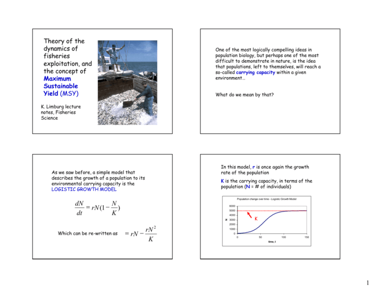
Theory of the
dynamics of
fisheries
exploitation, and
the concept of
Maximum
Sustainable
Yield (MSY)
One of the most logically compelling ideas in
population biology, but perhaps one of the most
difficult to demonstrate in nature, is the idea
that populations, left to themselves, will reach a
so-called carrying capacity within a given
environment…
What do we mean by that?
K. Limburg lecture
notes, Fisheries
Science
As we saw before, a simple model that
describes the growth of a population to its
environmental carrying capacity is the
LOGISTIC GROWTH MODEL
In this model, r is once again the growth
rate of the population
K is the carrying capacity, in terms of the
population (N = # of individuals)
Population change over time - Logistic Growth Model
N
dN
 rN (1  )
K
dt
6000
5000
N
4000
Which can be re-written as
rN 2
 rN 
K
K
3000
2000
1000
0
0
50
100
150
time, t
1
Population change over time - Logistic Growth Model
r = 0.08
K = 5000
N0 = 50
6000
5000
4000
N
The exact solution
to this model (so
that you can
program this in
Excel if you like) is
3000
2000
1000
0
0
50
100
150
time, t
Population change over time - Logistic Growth Model
6000
5000
r = 0.08
K = 5000
N0 = 1000
N
4000
K
Nt 
K  N 0  rt
1[
]e
No
3000
2000
1000
0
0
50
100
150
time, t
dB
B
 rB (1  )
dt
K
Population change over time - Logistic Growth Model
12000
This might represent the dynamics of an
unexploited fish stock…
10000
r = 0.1
K = 10000
N0 = 500
8000
N
(Do this for extra credit – and
remember what I said about order in
which computations are made!)
Just as we can track the changes in N
over time, we can also keep track of the
change in biomass (B), using the same
model but substituting B for N:
6000
4000
2000
0
0
50
100
150
time, t
To add exploitation onto this, we need
another “loss term” to represent the
harvest of biomass from the population.
We’ll call it Y, to represent yield.
dB
B
 rB (1  )
dt
K
Y
Theoretically, if a fishery is in steady state,
such that the yield (Y) is in balance with the
growth rate of the population, then
Y  rB(1 
B
)
K
2
Hypothetical fish population responds to
harvest regimes
If you can balance the harvest rate just at half
of the carrying capacity, then you will be
“cropping” the stock when it is growing the
fastest (in theory!)
harvest
assume logistic population growth
Biomass
growth  K
K
(King 1995)
In this graph, carrying capacity (K) is called
B
…and MSY stands for Maximum Sustainable Yield
Time
Slide courtesy C.M. Mayer
Biomass
small harvests,
slow growth near K
keeps biomass
oscillating around
K/2, highest growth
rate, leads to MSY
The models used to derive MSY are a
group called
SURPLUS PRODUCTION MODELS
And MSY itself is referred to as a
“biological reference point”
K
This means that it is a management criterion
that is derived from biological considerations
K/2
Oops…
Time
Other considerations include economics, social
welfare, etc. and can have other reference
points
3
Y  q f B,
Thinking about MSY in terms of fishing effort…
Recall that we can define harvesting in
terms of fishing effort, i.e.
Y  q f B,
Where
q = the “catchability” coefficient
f = fishing effort
(Q: what are some possible units??)
Note that Y/f is the catch per unit of
effort, or CPUE.
…is defined as the proportion of the
total stock caught by 1 unit of effort –
can vary due to a number of factors, so
must be measured (or assumed).
f, fishing effort, is the total amount of
effort used and should always be
standardized to a specific kind of effort
(e.g., hours of fishing with a particular gear
and vessel, horsepower, etc)
Y  f CPUE
Y q f B
Then B = CPUE/q .
If we substitute CPUE/q into the
equation of MSY, we get…
B
Y  rB(1  )
K
q, the catchability coefficient:
Substitute
CPUE/q in here
for B…
CPUE 

CPUE 
q 
 r
 1 

q
 CPUE 
q 

Y  rB (1 
B
)
K
CPUE when B = K
CPUE 

CPUE 
q 
 1 
f CPUE  r 

q
 CPUE 
q 

Divide through by CPUE…
4
q

CPUE  CPUE  f  CPUE  
r

If we divide by CPUE and collect terms, we get
CPUE = a - b f
r 
CPUE 
f   1 
q  CPUE 
Multiplying by fishing effort, f, and recalling
that Y = f x CPUE, we finally get
SCHAEFER’S MODEL:
Rearranging, it becomes
q

CPUE  CPUE  f  CPUE  
r

Y  af  bf 2
Once again, this is the equation of a straight line…
q

CPUE  CPUE  f  CPUE  
r

Y  af  bf 2
CPUE = a - b f
Q: What’s so great about the Schaefer model?
A: If we know f (the amount of fishing effort
used in a fishery), and we know Y (the yields at
different levels of f ), then we can estimate the
parameters a and b.
CPUE (= Y/f)
a = y-intercept = CPUE
CPUE q/r = -b (the slope)
x-intercept
= -a/b
Fishing effort (f)
(annihilation)
5
…we can solve for r.
Once we know a and b, we can apply it to the equation
for CPUE and get logistic growth parameters:
Y  af  bf 2
CPUE = a - b f
q

CPUE  CPUE  f  CPUE  
r

a
b
Y
Again, knowing this
relationship allows us
to estimate a and b…
f
If we know q, then we have an estimate
of B (because CPUE/q = B), and then
finally…
Another thing that comes out of the Shaefer
model is the level of effort corresponding to
MSY (fMSY).
This is found by differentiating the Shaefer
model with respect to f and solving for fMSY.
f MSY 
a
2b
(often you’ll see “E” instead of “f” for effort)
…and then, if we know
(or assume a value for)
q, we can solve for B,
the biomass of the fish
stock when it’s at
carrying capacity.
At least, in theory!
f MSY 
a
2b
It can be substituted into the
Shaefer model equation to solve for
MSY:
MSY  a (
a
a
 a2 a2
 a2


)  b( ) 2 
2b
2b
2b 4b
4b
Example: a = 10, b = -0.01. Then
MSY = -100/(-0.04) = 2500
6
Fisheries biologists also note that this is a guide
for knowing the level of effort that drives a
fishery “over the cliff” – i.e., is overfished. This
is defined as
foverfished = 2 fMSY
That is, a fish stock is overfished when
f 
a
b
Extensions of the MSY model
A number of variations on MSY modeling exist.
Among them is a model by Fox (1970)* that uses
an asymmetric effort curve, rather than the
Schaefer symmetric parabola:
Y
ln(CPUE )  ln( )  a  bf
f
* Fox, WW. 1970. Trans. American Fisheries Society 99: 80-88.
Y
ln(CPUE )  ln( )  a  bf
f
The FAO (Food and Agricultural Organization of
the United Nations) online manual of fisheries
management (Sparre and Venema, 1998, Chapter
9) states:
“…the choice between the two models becomes
important only when relatively large values of f
are reached. It cannot be proved that one of the
two models is superior to the other. You may
choose the one you believe is the most reasonable
in each particular case or the one which gives the
best fit to the data.”
(my italics)
7
These surplus yield models are very attractive,
because they don’t require nearly as much data as
other models (no need to determine ages, or sizes
of cohorts, no direct estimate of mortality, etc.)
However, as we’ll see later, these models have
caused a lot of grief to world fisheries.
Hence, it is likely to be adopted in situations
where data are scarce. (Q: is this a good thing?)
Photo: Candace Feit, The New York Times
Maximum Sustainable Yield: National and
International Definitions
1) The largest long-term average catch or yield that
can be taken from a stock or stock complex under
prevailing ecological and environmental conditions.
(US National Marine Fisheries Services (NOAA
Fisheries) strategic plan. Glossary of terms.
http://www.nmfs.noaa.gov/om2/glossary.html)
2) Maximum use that a renewable resource can sustain
without impairing its renewability through natural
growth or replenishment. (United Nations. Glossary
of environmental statistics.
http://unstats.un.org/unsd/environmentgl/ )
Literature cited.
King, M. 1995. Fisheries Biology, Assessment and
Management. Fishing News Books (Blackwell).
Sparre, P., and Venema, S.C. 1998. Introduction
to tropical fish stock assessment. Part 1. Manual.
FAO Fisheries Technical Paper. No. 306.1, Rev. 2.
Rome, FAO. 407p. (available online)
8