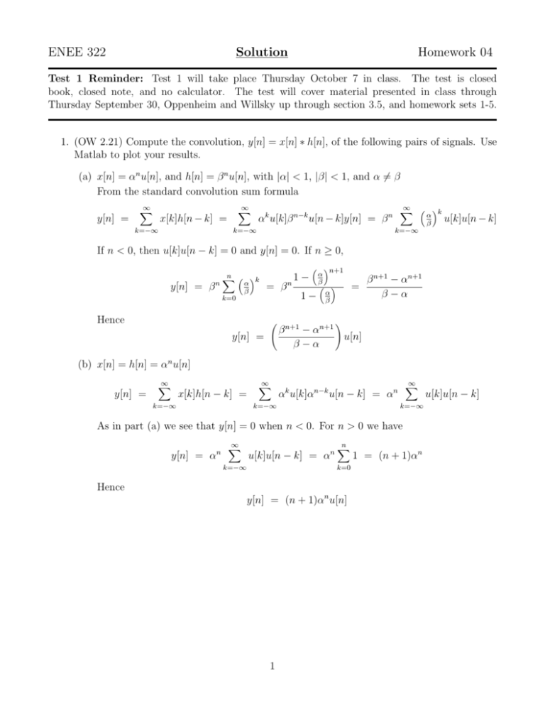
ENEE 322
Solution
Homework 04
Test 1 Reminder: Test 1 will take place Thursday October 7 in class. The test is closed
book, closed note, and no calculator. The test will cover material presented in class through
Thursday September 30, Oppenheim and Willsky up through section 3.5, and homework sets 1-5.
1. (OW 2.21) Compute the convolution, y[n] = x[n] ∗ h[n], of the following pairs of signals. Use
Matlab to plot your results.
(a) x[n] = αn u[n], and h[n] = β n u[n], with |α| < 1, |β| < 1, and α 6= β
From the standard convolution sum formula
y[n] =
∞
X
∞
X
x[k]h[n − k] =
k=−∞
αk u[k]β n−k u[n − k]y[n] = β n
k=−∞
∞ X
k
α
β
u[k]u[n − k]
k=−∞
If n < 0, then u[k]u[n − k] = 0 and y[n] = 0. If n ≥ 0,
y[n] = β
n
n X
k
α
β
= β
k=0
Hence
1−
n
n+1
1−
α
β
α
β
=
β n+1 − αn+1
β−α
β n+1 − αn+1
u[n]
β−α
!
y[n] =
(b) x[n] = h[n] = αn u[n]
y[n] =
∞
X
x[k]h[n − k] =
k=−∞
∞
X
αk u[k]αn−k u[n − k] = αn
k=−∞
∞
X
k=−∞
As in part (a) we see that y[n] = 0 when n < 0. For n > 0 we have
y[n] = αn
∞
X
u[k]u[n − k] = αn
k=−∞
n
X
k=0
Hence
y[n] = (n + 1)αn u[n]
1
1 = (n + 1)αn
u[k]u[n − k]
α = 0.750, β = 0.250
α = 0.750
1
1.6
1.4
0.8
1.2
ya[n]
yb[n]
0.6
1
0.8
0.4
0.6
0.4
0.2
0.2
0
−5
0
5
10
0
−5
15
5
n
α = 0.450, β = 0.350
α = 0.450
0.8
0.8
0.6
0.6
10
15
10
15
10
15
yb[n]
1
ya[n]
1
0.4
0.4
0.2
0.2
0
−5
0
n
0
5
10
0
−5
15
0
5
n
n
α = 0.900, β = 0.100
α = 0.900
1
3.5
3
0.8
2.5
yb[n]
ya[n]
0.6
2
1.5
0.4
1
0.2
0.5
0
−5
0
5
10
0
−5
15
n
0
5
n
2
2. For the following pairs of signals, use the convolution integral to find the response y(t) of the
LTI system with impulse response h(t) to the input x(t). Plot your results using Matlab.
(a) x(t) = u(t), and h(t) = e−t u(t).
y(t) =
Z
∞
−∞
x(τ )h(t − τ )dτ =
Z
∞
−∞
x(t − τ )h(τ )dτ =
Z
∞
−∞
u(t − τ )e−τ u(τ )dτ
When t < 0, the curves do not overlap so y(t) = 0. For t > 0,
y(t) =
t
Z
0
e−τ dτ = 1 − e−t
Hence
i
h
y(t) = 1 − e−t u(t)
(b) x(t) = e−αt u(t), and h(t) = e−βt u(t), with α > 0, β > 0, and α 6= β
y(t) =
Z
∞
−∞
x(τ )h(t − τ )dτ
When t < 0, there is no overlap so y(t) = 0. For t > 0,
y(t) =
Z
t
e−ατ e−β(t−τ ) dτ = e−βt
0
Z
t
eτ (β−α) dτ =
h
i
e−βt et(β−α) − 1
β−α
0
Hence,
y(t) =
e−αt − e−βt
u(t)
β−α
α = 0.50, β = 1.00
1
0.5
0.45
0.4
0.7
0.35
0.6
0.3
yb(t)
0.8
0.5
0.25
a
y (t)
0.9
0.4
0.2
0.3
0.15
0.2
0.1
0.1
0.05
0
−2
−1
0
1
2
3
4
0
−2
5
t
0
2
4
t
3
6
8
10
(c) x(t) = u(t + 3) − 2u(t) + u(t − 3), and h(t) = u(t + 1) − u(t − 1)
y(t) =
Z
∞
−∞
∞
Z
x(τ )h(t − τ )dτ =
−∞
x(τ ) [u(t − 1 − τ ) − u(t + 1 − τ )] dτ
Will need to evaluate this integral for various ranges of t. Drawing pictures will help.
h(τ)
x(τ)
h(t-τ)
3
-3
τ
0
-1 0 1
τ
t-1
t+1 τ
Region 1: When t + 1 ≤ −3 there will not be any overlap, so y(t) = 0 when t ≤ −4.
Region 2: When t − 1 ≤ −3 and t + 1 ≥ −3 we have
3
t-1 -3 t+1
τ
0
and the resulting integral is
Z
y(t) =
t+1
−3
1dτ = [t]t+1
−3 = t + 4
Hence y(t) = t + 4 when −4 ≤ t ≤ −2.
Region 3: When t − 1 ≥ −3 and t + 1 ≤ 0, we have
3
-3 t-1
τ
t+1 0
and the resulting integral is
y(t) =
Z
t+1
t−1
1dτ = [t]t+1
t−1 = 2
Hence y(t) = 4 when −2 ≤ t ≤ −1.
Region 4: When t − 1 ≤ 0 and t + 1 ≤ 2
3
-3
t-1
τ
t+1
and the resulting integral is
y(t) =
Z
0
t−1
dτ −
Z
0
t+1
dτ = [0 − (t − 1)] − [(t + 1) − 0] = −2t
Hence y(t) = −2t when −1 ≤ t ≤ 1.
Region 5: When t − 1 ≥ 0 and t + 1 ≤ 3, we have
3
-3
0 t-1
4
t+1
τ
and the resulting integral is
y(t) = −
Z
t+1
t−1
1dτ = − [t]t+1
t−1 = −[(t + 1) − (t − 1)] = −2
Hence y(t) = −2 when 1 ≤ t ≤ 2.
Region 6: When t − 1 ≤ 3 and t + 1 ≥ 3, we have
3
-3
0
t-1
t+1
and the resulting integral is
y(t) = −
Z
3
t−1
dτ = − [t]3t−1 = −[3 − (t − 1)] = t − 4
Hence y(t) = t − 4 when 2 ≤ t ≤ 4
Region 7: Finally for t ≥ 4 there is no overlap so y(t) = 0 for t > 4.
y(t) =


0





t+4





2

−2t



−2





t
−
4




0
t ≤ −4
−4 ≤ t ≤ −2
−2 ≤ t ≤ −1
−1 ≤ t ≤ 1
1≤t≤2
2≤t≤4
t≥4
2
1.5
1
yc(t)
0.5
0
−0.5
−1
−1.5
−2
−6
−4
−2
0
t
5
2
4
6
3. Each of these signals is the impulse response of an LTI system. Determine whether each of
these LTI systems is causal and/or stable. Justify your answers.
(a) h[n] = 2n u[1 − n]
Since h[−1] 6= 0, the system is Noncausal
∞
X
|h[n]| =
n=−∞
1
X
2n =
n=−∞
∞
X
(0.5)m = 2 +
m=−1
1
= 4 < ∞
1 − 0.5
Hence the system is Stable
(b) h(t) = e−|t|
Since h(t) is nonzero for t < 0, the systems is Noncausal
Z
∞
−∞
|h(t)| dt =
Z
∞
−|t|
e
dt = 2
−∞
Z
0
∞
e−t dt = −2 [0 − 1] = 2 < ∞
Hence the system is Stable
(c) h(t) = te−t u(t)
Since h(t) = 0 for all t < 0, the systems is Causal
Z
∞
−∞
|h(t)| dt =
Z
0
∞
∞
te−t dt = −(t + 1)e−t because te−t → 0 as t → ∞. Hence the system is Stable
6
0
= 1 < ∞
4. (OW 1.42)
(a) Is the series interconnection of two linear time-invariant systems always a linear timeinvariant system? Justify your answer.
Yes. Consider two systems S1 and S2 connected in series. Assume that if x1 (t) and x2 (t)
are inputs to S1 , then the outputs are y1 (t) and y2 (t), respectively. Also, assume that if
y1 (t) and y2 (t) are inputs to S2 , then the outputs are z1 (t) and z2 (t), respectively. Since
S1 is linear we know that for constants a, b
S
1
ax1 (t) + bx2 (t) −→
ay1 (t) + by2 (t)
Since S2 is linear we know that
S
2
ay1 (t) + by2 (t) −→
az1 (t) + bz2 (t)
Hence
S S
1 2
ax1 (t) + bx2 (t) −→
az1 (t) + bz2 (t)
so the interconnection of two LTI systems is itself an LTI system.
(b) Is the series interconnection of two nonlinear systems a nonlinear system? Justify your
answer.
Consider the following two nonlinear systems
y(t) = x(t) + 1
z(t) = y(t) − 1
If they are connected in series, the z(t) = x(t) which is linear. Hence the interconnection
of two nonlinear systems can be linear.
(c) Consider three systems with the following input-output relationships which are connected
in series as depicted below.
System 1:
System 2:
System 3:
(
x[n/2],
n even
0,
n odd
1
y[n] = x[n] + 2 x[n − 1] + 14 x[n − 2]
y[n] = x[2n]
y[n] =
x[n]
System 1
System 2
y[n]
System 3
Find the input-output relationship for the overall interconnected system. Is this system
linear? Is it time-invariant?
Name the output of system 1 w[n] and the output of suystem 2 z[n]. Then
1
1
1
y[n] = z[2n] = w[2n] + w[2n − 1] + w[2n − 2] = x[n] + x[n − 1]
2
4
4
The overall system is LTI.
7
Additional Problems. Do Not Turn In!!
5. (OW 2.40) An LTI systems has the following input-output relationship
t
Z
y(t) =
e−(t−τ ) x(τ − 2)dτ
−∞
(a) What is the impulse response, h(t), for this system.
Recall that h(t) = y(t) when x(t) = δ(t), so
t
Z
h(t) =
−∞
(
=
e−(t−τ ) δ(τ − 2)dτ
0
t<2
−(t−2)
e
t>2
h(t) = e−(t−2) u(t − 2)
(b) Determine the response of the system, when the input is:
x(t)
1
-1
0
1
2 t
Sketching x(t − τ ) and h(τ ),
x(t-τ)
h(τ)
t-2
2 t+1
τ
we see that y(t) = 0 for t + 1 < 2. When t − 2 < 2 and t + 1 > 2
y(t) =
Z
t+1
2
t+1
e−(τ −2) dτ = −e−(τ −2) 2
h
= −e−(t−1) + e0 = 1 − e−(t−1)
i
When t − 2 > 2
y(t) =
Z
t+1
t−2
t+1
e−(τ −2) dτ = −e−(τ −2) Hence
y(t) =



0

 h
h
t−2
t ≤ 1
−(t−1)
1−e
i



 [1 − e−3 ] e−(t−4)
8
i
= −e−(t−1) + e−(t−4) = 1 − e−3 e−(t−4)
1 < t ≤ 4
4 < t
6. (OW 2.43) One of the most important properties of convolution, in both continuous and
discrete time, is the associativity property. In this problem, we will check and illustrate this
property.
(a) Prove the equality
[x(t) ∗ h(t)] ∗ g(t) = x(t) ∗ [h(t) ∗ g(t)]
by showing that both sides of the equation equal
Z
∞
−∞
Z
∞
−∞
x(τ )h(σ)g(t − τ − σ)dτ dσ
For the LHS we have
Z
x(t) ∗ h(t) =
∞
−∞
Z ∞
[x(t) ∗ h(t)] ∗ g(t) =
=
−∞
Z ∞
=
Z
−∞
∞
−∞
Z ∞
[x(t) ∗ h(t)] ∗ g(t) =
−∞
x(τ )h(t − τ )dτ
[x ∗ h] (λ)g(t − λ)dλ
Z
Z
∞
−∞
∞
x(τ )h(λ − τ )dτ g(t − λ)dλ
−∞
Z ∞
−∞
x(τ )h(λ − τ )g(t − λ)dτ dλ
x(τ )h(σ)g(t − τ − σ)dτ dσ
where we have made the change of variables σ = λ − τ . Similarly, for the RHS
h(t) ∗ g(t) =
Z
x(t) ∗ [h(t) ∗ g(t)] =
Z
=
x(t) ∗ [h(t) ∗ g(t)] =
∞
−∞
∞
−∞
Z ∞
−∞
∞
Z
−∞
h(σ)g(t − σ)dσ
x(τ ) [h ∗ g] (t − τ )dτ
x(τ )
Z
∞
−∞
Z
∞
−∞
h(σ)g(t − τ − σ)dσ dτ
x(τ )h(σ)g(t − τ − σ)dτ dσ
(b) Consider two LTI systems with impulse responses h1 [n] and h2 [n] which are cascaded as
shown below
1 n
h1 [n] = −
u[n]
2
1
h2 [n] = u[n] + u[n − 1]
2
h2 [n]
h1 [n]
1
x[n]
h1 [n]
w[n]
h2 [n]
1
y[n]
-2 -1 0
Let the input signal be x[n] = u[n]
9
2
4 n
-2 -1 0 1 2 3 4 n
i. Compute y[n] = (x[n] ∗ h1 [n]) ∗ h2 [n], i.e., first compute w[n] = x[n] ∗ h1 [n] and then
compute y[n] = w[n] ∗ h2 [n].
w[n] =
∞
X
∞
X
x[n − k]h1 [k] =
k=−∞
u[n − k] −
k=−∞
1
2
k
u[k]
Clearly when n < 0 we have w[n] = 0, so
w[n] =
y[n] =
=
"
n X
k=0
∞
X
1
−
2
k #
"
2
1
u[n] =
1− −
3
2
n+1 #
u[n]
w[k]h2 [n − k]
k=−∞
∞
X
k+1
2
1
u[k] u[n − k] + u[n − 1 − k]
1 − − 12
2
k=−∞ 3
For n <= −1, we see that y[n] = 0, and y[0] = 1. For n ≥ 1,
n
2X
1
1− −
y[n] =
3 k=0
2
"
k+1 #
X
1 n−1
1
+
1− −
3 k=0
2
"
n
2
2X
1
=
(n + 1) −
−
3
3 k=0
2
n
1X
1
−
3 k=0
2
1 1
+ n
3 3
2
=
(n + 1) +
3
2
=
(n + 1) +
3
y[n] = (n + 1)
k+1
k+1 #
X
1
1 n−1
1
+ n−
−
3
3 k=0
2
n
1
1 X
1
+ n−
−
3
3 m=1
2
k
k+1
m
Hence
y[n] = (n + 1) u[n]
ii. Compute y[n] = x[n] ∗ (h1 [n] ∗ h2 [n]), i.e., first compute g[n] = h1 [n] ∗ h2 [n] and then
compute y[n] = x[n] ∗ g[n].
g[n] =
∞
X
∞ X
h1 [k]h2 [n − k] =
k=−∞
k=−∞
−
1
2
k
1
u[k] u[n − k] + u[n − 1 − k]
2
From the above figures, we see that g[n] = 0 for n <= −1, and g[0] = 1. For n ≥ 1,
g[n] =
n X
k=0
1
−
2
k
X
1 n−1
1
+
−
2 k=0
2
k
2
1 n+1
1
1
=
1− −
+
1− −
3
2
3
2
n+1
n
2
1
1
1
= 1−
−
−
−
3
2
3
2
g[n] = 1
"
10
#
n Hence g[n] = u[n]. Now
y[n] =
∞
X
x[k]g[n − k] =
k=−∞
∞
X
u[k]u[n − k] =
k=−∞
n
X
1 = (n + 1)u[n]
k=0
The answers to (i) and (ii) should be identical, illustrating the associativity property of
discrete time convolution.
(c) Now consider two the cascade of two LTI systems with
h1 [n] = sin(8n)
h2 [n] = an u[n],
|a| < 1
x[n] = δ[n] − aδ[n − 1]
Determine the output y[n]. (Hint: The use of the associative and commutative properties
of convolution should greatly facilitate the solution.)
Note that
y[n] = x[n] ∗ (h1 [n] ∗ h2 [n]) = x[n] ∗ (h2 [n] ∗ h1 [n]) = (x[n] ∗ h2 [n]) ∗ h1 [n]
Also
x[n] ∗ h2 [n] = (δ[n] − aδ[n − 1]) ∗ h2 [n]
= h2 [n] − ah2 [n − 1]
= an u[n] − a an−1 u[n − 1]
= an (u[n] − u[n − 1])
x[n] ∗ h2 [n] = δ[n]
Hence
y[n] = (x[n] ∗ h2 [n]) ∗ h1 [n] = δ[n] ∗ sin(8n) = sin(8n)
11