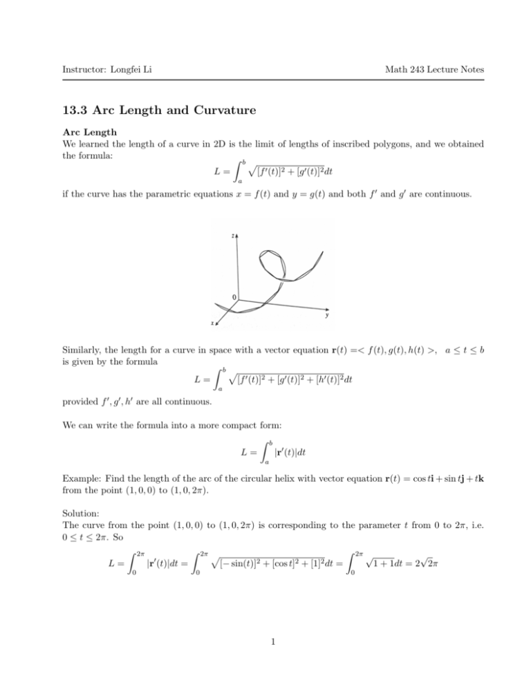
Instructor: Longfei Li
Math 243 Lecture Notes
13.3 Arc Length and Curvature
Arc Length
We learned the length of a curve in 2D is the limit of lengths of inscribed polygons, and we obtained
the formula:
Z bp
L=
[f 0 (t)]2 + [g 0 (t)]2 dt
a
if the curve has the parametric equations x = f (t) and y = g(t) and both f 0 and g 0 are continuous.
Similarly, the length for a curve in space with a vector equation r(t) =< f (t), g(t), h(t) >, a ≤ t ≤ b
is given by the formula
Z bp
L=
[f 0 (t)]2 + [g 0 (t)]2 + [h0 (t)]2 dt
a
provided
f 0 , g 0 , h0
are all continuous.
We can write the formula into a more compact form:
Z
L=
b
|r0 (t)|dt
a
Example: Find the length of the arc of the circular helix with vector equation r(t) = cos ti + sin tj + tk
from the point (1, 0, 0) to (1, 0, 2π).
Solution:
The curve from the point (1, 0, 0) to (1, 0, 2π) is corresponding to the parameter t from 0 to 2π, i.e.
0 ≤ t ≤ 2π. So
Z 2π
Z 2π p
Z 2π
√
√
0
2
2
2
[− sin(t)] + [cos t] + [1] dt =
1 + 1dt = 2 2π
L=
|r (t)|dt =
0
0
0
1
Figure 1: This is the graph that the equation r(t) = cos ti + sin tj + tk from
the point (1, 0, 0) to (1, 0, 2π) represents
A single curve C can be represented by a vector equation
r(t) =< f (t), g(t), h(t) >,
and the vector equation is called a parametrization of the curve C.
Remark: Parametrizations of a curve is not unique.
For instance, the twisted cubic
r(t) =< t, t2 , t3 >, 1 ≤ t ≤ 2
can also be represented by the parametrization
r(u) =< eu , e2u , e3u >, 0 ≤ u ≤ ln 2
provided t = eu .
Remark: Reparametrize a curve is similar to change of variables.
The arc length arises naturally from the shape the curve and does not depend on parametrization.
Arc Length Function: Suppose C is curve given by a vector function
r(t) = f (t)i + g(t)j + h(t)k,
a≤t≤b
where r0 is continuous and C is traversed once as t increases from a to b.
Definition The arc length function s is defined by
Z t
s(t) =
|r0 (u)|du
a
Remark: s(t) is the arc length of the part C between r(a) and r(t).
According to the Fundamental Theorem of Calculus, we have
ds
= |r0 (t)|
dt
Often times, it’s useful to parametrize a curve with respect to its arc length because arc length is
independent on parametrizations.
2
Example: Reparametrize the line r(t) =< 2t, 1 − 3t, 5 + 4t > with respect to arc length measured from
(0, 1, 5) in the direction of increasing t.
Solution:
The arc length measured from the point (0, 1, 5) corresponding to t = 0. To reparametrize the curve
w.r.t. the arc length, we need the relation between s and t. Since
Z t√
Z t
√
√
ds
0
0
= |r (t)| = | < 2, −3, 4 > | = 29 ⇒ s(t) =
|r (u)|du =
29du = 29t
dt
0
0
Therefore,
s
t= √ ,
29
and the reparametrization is obtained by substituting for t
s
s
s
r(s) =< 2 √ , 1 − 3 √ , 5 + 4 √ >
29
29
29
Curvature
A parametrization r(t) is called smooth on an interval I if r0 (t) is continuous and nonzero.
A curve is called smooth if it has a smooth parametrization (No sharp corners or cusps; tangent vector
turns smoothly.)
Note that when C is nearly straight, the direction of tangent vector changes slowly; when C bends or
twists more sharply, the direction of tangent vector changes more quickly.
Curvature at a point is defined to measure how quickly the curve changes direction at that point.
Definition: The curvature of a curve is
dT κ=
ds
where T is the unit tangent vector. Remark: differentiate with respect to arc length.
It’s easier to compute a curvature if it is expressed in terms of t instead of s.
3
From Chain Rule:
dT
dT ds
dT
dT . ds
=
⇒
=
dt
ds dt
ds
dt dt
We know
ds
= |r0 (t)|,
dt
So
κ(t) =
|T0 (t)|
|r0 (t)|
The curvature of the curve given by the vector function r:
κ(t) =
|r0 (t) × r00 (t)|
|r0 (t)|3
(Read theorem 10 in the textbook for the proof)
For a plane curve, y = f (x), curvature can be given by
κ(x) =
|f 00 (x)|
[1 + (f 0 (x))2 ]3/2
(This formula is derived from the vector equation formula by using r =< x, f (x), 0 >)
Example:
Find the curvature of the curve given by r(t) =< a cos t, a sin t, 0 >.
Solution:
r0 (t) =< −a sin t, a cos t, 0 >
r00 (t) =< −a cos t, −a sin t, 0 >
So
|r0 (t) × r00 (t)| = |(a2 sin2 t + a2 cos2 t)k| = |a2 k| = a2
and
|r0 (t)| = a
Therefore, from the formula given by the vector function:
κ(t) =
|r0 (t) × r00 (t)|
a2
1
=
=
|r0 (t)|3
a3
a
Remark: r(t) in this example represents a circle with radius a. The results shows larger circles have
smaller curvature while smaller circles have lager curvature.
4
The Normal and Binormal Vectors
Sometimes it’s useful to have a moving reference frame.
Remark: Reference frame is a set of orthogonal vectors
r0 (t)
. We need a vector orthogonal to
|r0 (t)|
0
T. Recall from the example of previous lecture that |T| = 1 ⇒ T · T = 0, i.e., T0 is orthogonal to T.
T0 is not necessarily a unit vector, but if r is smooth, and r0 6= 0, we can find the corresponding unit
vector of T0 .
We have already introduced the unit tangent vector T(t) =
Definition: The principle unit normal vector is defined by
N(t) =
T0 (t)
|T0 (t)|
Remark: N(t) indicates the direction where the curve is turning.
We need another unit vector that is orthogonal to both T and N to get a reference frame in 3D space.
Definition: The binormal vector is defined by
B(t) = T(t) × N(t)
Remark: B is a unit vector because |B| = |T × N| = |T||N| sin π2 = 1
We call the plane containing N and B at a point P the normal plane of the curve at P (It consists of
all lines orthogonal to T)
Formula Summary:
T(t) =
r0 (t)
,
|r0 (t)|
N(t) =
T0 (t)
,
|T0 (t)|
B(t) = T(t) × N(t)
dT |T0 (t)|
|r0 (t) × r00 (t)|
κ(t) = =
= 0
ds
|r (t)|
|r0 (t)|3
5