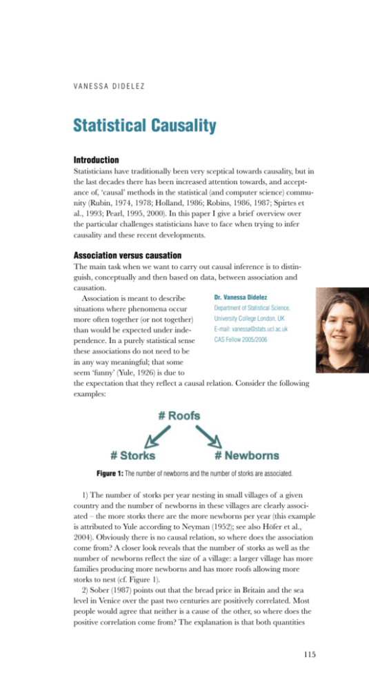
V anessa D idele z
Statistical Causality
Introduction
Statisticians have traditionally been very sceptical towards causality, but in
the last decades there has been increased attention towards, and acceptance of, ‘causal’ methods in the statistical (and computer science) community (Rubin, 1974, 1978; Holland, 1986; Robins, 1986, 1987; Spirtes et
al., 1993; Pearl, 1995, 2000). In this paper I give a brief overview over
the particular challenges statisticians have to face when trying to infer
causality and these recent developments.
Association versus causation
The main task when we want to carry out causal inference is to distinguish, conceptually and then based on data, between association and
causation.
Dr. Vanessa Didelez
Association is meant to describe
Department of Statistical Science,
situations where phenomena occur
University College London, UK
more often together (or not together)
E-mail: vanessa@stats.ucl.ac.uk
than would be expected under indeCAS Fellow 2005/2006
pendence. In a purely statistical sense
these associations do not need to be
in any way meaningful; that some
seem ‘funny’ (Yule, 1926) is due to
the expectation that they reflect a causal relation. Consider the following
examples:
Figure 1: The number of newborns and the number of storks are associated.
1) The number of storks per year nesting in small villages of a given
country and the number of newborns in these villages are clearly associated – the more storks there are the more newborns per year (this example
is attributed to Yule according to Neyman (1952); see also Höfer et al.,
2004). Obviously there is no causal relation, so where does the association
come from? A closer look reveals that the number of storks as well as the
number of newborns reflect the size of a village: a larger village has more
families producing more newborns and has more roofs allowing more
storks to nest (cf. Figure 1).
2) Sober (1987) points out that the bread price in Britain and the sea
level in Venice over the past two centuries are positively correlated. Most
people would agree that neither is a cause of the other, so where does the
positive correlation come from? The explanation is that both quantities
115
Statistical Causality
have steadily increased over time due to their respective local conditions
which are not further related to each other (cf. Figure 2). Hence it is two
unrelated time trends that induce an association.
Figure 2: Bread price in Britain and water level in Venice both exhibit a time trend.
There is no single agreed on definition of causality in the statistical and
philosophical literature. In the statistical literature one can distinguish at
least four broad approaches: (i) probabilistic causality, reducing the question of causality to probabilistic statements among suitably defined events;
(ii) counterfactual causality, addressing the question of “what if something
had been different in the past”; (iii) structural models, assuming that the
system of interest is driven by stable (stochastic) mechanisms this approach
addresses under which condition these mechanisms can be uncovered;
(iv) decision theory, addressing the question of making optimal decisions
under uncertainty.
Maybe except for (i) all of these approaches deal, more or less explicitly,
with causation as the effect of an intervention in one (or more) variable(s)
on some response variable. Typically, scientists are interested in causal
relations because they want to intervene in some sense, to prevent diseases or to
make life easier etc. Some examples:
1) It is well known that the increase of CFC use has been accompanied
by ozone depletion, i.e. there is a clear association between the two. The
underlying photochemical processes are by now studied and understood
well enough to say that CFC is the cause of the ozone depletion. Hence
we would expect that reducing the level of CFC (by some intervention!) will slow down or even reverse the ozone depletion. The Montreal
Protocol signed by 43 nations in 1987 could be regarded as such an intervention to reduce and phase out the use of CFC.
2) We can be pretty sure that manipulating the number of storks in a
village, e.g. setting it to zero by killing them, will not change the number
of newborns in that same village – this association is not causal.
We now turn to the question of why associations can be observed
without an underlying causal relation. A cause X and a response Y will
be associated if X is indeed causal for Y but not necessarily vice versa,
as demonstrated with the above examples. The following are alternative
explanations.
Common Cause – Confounding. If X and Y have a common cause,
as in the storks/newborns example, they can be associated without being
causally related at all. The presence of a common cause is often called
confounding.
Reverse Causation. In reality, Y might be the cause of X and not, as
we think, vice versa. For example if X is the homocysteine level and Y is
coronary heart disease then it could be that existing atherosclerosis leads
to increased levels of homocysteine and not vice versa.
116
Statistical Causality
Time Trends. X and Y may only be associated because they are the
results of two processes with time trends without these time trends being
related to each other, as for example the bread price and water level in
Venice.
Feedback. X and Y may be associated because they instigate each
other. As an example consider alcohol abuse and social problems: does a
person drink due to social problems, like problems in his job, or are such
problems the consequence of alcohol abuse or both?
Of course one should never forget that observed associations may
just be due to coincidence. Also, it would be presumptuous to claim that
the above list is complete; there may be other reasons that scientists and
philosophers have not thought of yet.
Methods to assert causation
If we want to investigate what happens when we manipulate a variable, then an obvious method is to actually carry out such manipulations
and observe the result. This is what is done in experimental studies. For
instance in a clinical trial, patients are randomly allocated either to the
treatment group or to the non-treatment (control) group. This random
allocation ensures that X is not associated (except by coincidence) with
anything that is not a consequence of X rendering most of the above
explanations for association without causation very unlikely. In addition,
clinical studies are often ‘double blind’ meaning that neither the patients
nor the doctors or nurses know who is in which group. This is secured
by formulating the investigational drug and the control (either a placebo
or an established drug) to have identical appearance. Hence it is ensured
that the psychological effect is the same in both groups. In other areas it is
more difficult to design good experiments, but researchers are inventive,
for instance sociologists when investigating discrimination by faking the
names on CVs (Bertrand and Mullainathan, 2003).
In many subjects, in particular in epidemiology, it is impossible to carry
out experiments. For instance if the ‘cause’ is smoking behaviour, alcohol
consumption or education, we cannot randomly allocate subjects to
different groups. Instead we have to make do with data on the behaviour
as it is, but this will typically mean having to deal with confounding as, for
example, smokers are likely to exhibit a life style that is different also in
other respects from that of non-smokers (cf. Figure 3).
So how do we infer causation from non-experimental data? In some
circumstances when a thorough knowledge of the subject matter is available one can identify the confounders and measure them in addition to
the X and Y variable of interest. The causal effect can then be assessed
within every level of the confounders, i.e. based on stratification. This
yields valid causal inference if a sufficient set of confounders is used.
There are many problems with this approach: one can never be sure
about what the relevant confounders are and even then, there may be
many different ways of measuring them; in addition, typical confounders
are prone to errors, e.g. self-reported alcohol consumption is known to
be unreliable. Hence, unlike experimental studies, causal inference from
epidemiological data rests on a certain prior knowledge of the system
under investigation. Graphical representations of background knowledge
have been suggested to facilitate this task (Pearl 1995, 2000). Such graphs
117
Statistical Causality
represent the conditional independencies (i.e. purely probabilistic relations) but can, under certain assumptions, be informative about causal
relations.
Figure 3: The problem of confounding in Epidemiology.
The role of time
Recall that confounding is only one of the reasons why we may observe
associations without the desired causation. Reverse causation, time trends
and feedback all involve time but it is even more difficult to ‘adjust for
time’ than the above ‘adjustment for confounding’.
First of all we obviously need to have data over time – usually from
so-called longitudinal studies. Secondly, we must be careful not to adjust for
so-called mediating (or intermediate) variables. To explain this, consider the
simple example in Figure 4.
Figure 4: Example for an intermediate variable.
The effect of smoking on developing lung cancer can plausibly be
assumed to be mediated by the ensuing amount of tar deposit in the
lungs – note that passive smoking may also result in tar in the lungs.
The above graph even suggests that once the amount of tar is known,
cancer risk and smoking are independent. If we mistakenly think of ‘tar
deposit’ as a confounder and adjust for it, we may therefore wrongly find
that there is no effect of smoking on lung cancer. This is because within
every given level of ‘tar deposit’, whether the person is smoking or passive
smoking makes no difference anymore to her probability of developing
lung cancer. It is well known among epidemiologists that adjusting for
mediating variables can ‘hide’ the causal effect in which we are interested
(Weinberg, 1993).
Thirdly, we must further be aware that in longitudinal settings certain
variables can be confounders for some treatments and intermediates for
others. For example, consider a study where patients with operable breast
cancer receive repeated cycles of chemotherapy, the number of which
depends on the development of the size of the tumour as monitored by
palpation and imaging methods, and the outcome is whether or not there
are any malignant cells remaining at surgery (cf. Minckwitz et al., 2005).
Obviously the tumour size is a good predictor of the outcome. The aim of
this study is to identify the number of tumour cycles required to destroy
118
Statistical Causality
all cancer cells. The problem is that the tumour size is a mediating variable of earlier chemotherapy. Hopefully, once the first chemotherapy cycle
has been given, the tumour should start to decrease. However, tumour
size is also a confounder, because if the tumour is still large, more chemotherapy cycles might be given, or in bad cases the therapy is interrupted
and surgery takes place immediately (cf. Figure 5, where only two stages
are represented).
Figure 5: ‘Size of tumour’ is a mediating variable for first chemotherapy and a confounder for
second chemotherapy.
The solution to this problem goes back to the groundbreaking work
of Robins (1986, 1987) who showed that the key principle is to adjust at
any point in time only for past observations and then ‘piece together’ the
results for the individual time points to obtain the overall causal effect (cf.
also Dawid and Didelez, 2005). This method is very plausible but still not
widely understood. Also, it still has to cope with several other problems
such as being computationally very involved, especially when measurements are taken continuously over time.
Conclusions
Statisticians can contribute to discovering causal relations in a variety
of fields. In fact many old and recent advances in areas like technology
and medicine are due to thorough experimentation, data collection and
analysis. However, it seems that such advances are more pronounced
in subjects where experiments can easily be carried out than in other
subjects, e.g. in psychology, nutrition science or politics. These problems
are clearly reflected in the challenges that statisticians face, as I have
outlined in this article. It is much more difficult to infer causation from
non-experimental data and it always requires prior background knowledge, e.g. on what could be potential confounders, and it often needs
careful and patient observations over time.
References
Bertrand, M., Mullainathan, S.: “Are Emily and Greg more employable than Lakisha and
Jamal? A field experiment on labor market discrimination”. NBER working paper series no.
9873. Cambridge: National Bureau of Economic Research, 2003.
Dawid, A.P., and Didelez, V. “Identifying the consequences of dynamic treatment strategies”. Research Report No. 262, Department of Statistical Science, University College
London, 2000.
Höfer, T., Przyrembel, H., Verleger, S. “New evidence for the theory of the stork”. Paediatric
and Perinatal Epidemiology 18, 2004, pp. 88–92.
Holland, P.W. “Statistics and causal inference”. Journal of the American Statistical Association 81,
1986, pp. 945–60.
Minckwitz, G., Raab, G., Caputo, A., Schütte, M., Hilfrich, J., Blohmer, J.U., Gerber,
B., Costa, S.D., Merkle, E., Eidtmann, H., Lampe, D., Jackisch, C., du Bois, A., and
119
Statistical Causality
Kaufman, M.: “Doxorubicin with cylophosphamide followed by docetaxel every 21 days
compared with doxorubicin and docetaxel every 14 days as preoperative treatment in
operable breast cancer”. Journal of Clinical Oncology 23, 2005, pp. 2676–85.
Neyman, J.: Lectures and Conferences on Mathematical Statistics and Probability, second edition,
Graduate School U.S. Department of Agriculture, Washington, 1952.
Pearl, J.; “Causal diagrams for empirical research”. Biometrika 82, 1995, pp. 669–710.
Pearl, J.: Causality. Cambridge University Press, 2000.
Robins, J.M.: “A new approach to causal inference in mortality studies with sustained exposure periods – application to control of the healthy worker survivor effect”. Mathematical
Modelling 7, 1986, pp. 1393–1512.
Robins, J.M.: Addendum to “A new approach to causal inference in mortality studies with
sustained exposure periods – application to control of the healthy worker survivor
effect”. Computers and Mathematics, with Applications 14, 1987, pp. 923–45.
Rubin, D.B.: “Estimating causal effects of treatments on randomized and non-randomized
studies”. Journal of Educational Psychology 66, 1974, pp. 688–701.
Rubin, D.B.: “Bayesian inference for causal effects: the role of randomization”. Annals of
Statistics 6, 1978, pp. 34–58.
Sober, E.: “The principle of the common cause”. In J. Fetzer (ed.), Probability and Causation:
Essays in Honor of Wesley Salmon. Dordrecht, Reidel, 1987, pp. 211–29.
Sprites, P., Glymour, C. and Scheines, R.: Causation, Prediction and Search. New York, SpringerVerlag, 1993. 2nd edition published in 2000.
Weinberg, C.: “Towards a clearer definition of confounding”. American Journal of Epidemiology
137, 1993, pp. 1–8.
Yule, G.U.: “Why do we sometimes get nonsensical relations between time series? A study of
sampling and the nature of time series”. Journal of the Royal Statistical Society 89, 1926, pp.
1–64.
120