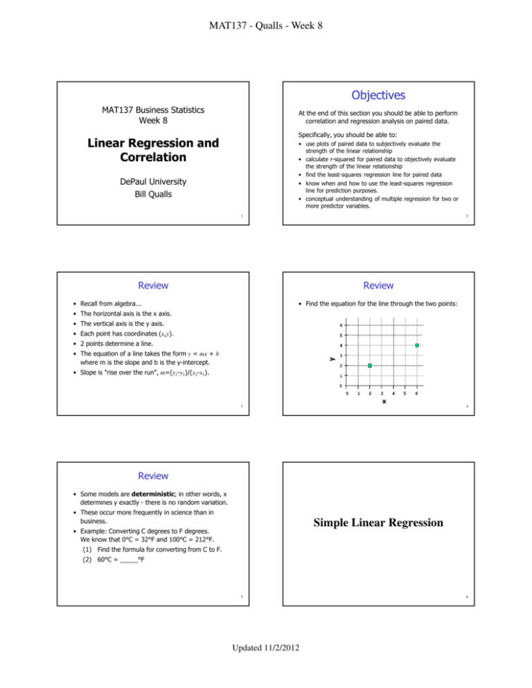
MAT137 - Qualls - Week 8
Objectives
MAT137 Business Statistics
Week 8
At the end of this section you should be able to perform
correlation and regression analysis on paired data.
Specifically, you should be able to:
Linear Regression and
Correlation
• use plots of paired data to subjectively evaluate the
strength of the linear relationship
• calculate r-squared for paired data to objectively evaluate
the strength of the linear relationship
• find the least-squares regression line for paired data
• know when and how to use the least-squares regression
line for prediction purposes.
• conceptual understanding of multiple regression for two or
more predictor variables.
DePaul University
Bill Qualls
1
2
Review
Review
• Recall from algebra...
• Find the equation for the line through the two points:
• The horizontal axis is the x axis.
• The vertical axis is the y axis.
• Each point has coordinates (x,y).
• 2 points determine a line.
• The equation of a line takes the form y = mx + b
where m is the slope and b is the y-intercept.
• Slope is "rise over the run", m=(y2-y1)/(x2-x1).
3
4
Review
• Some models are deterministic; in other words, x
determines y exactly - there is no random variation.
• These occur more frequently in science than in
business.
Simple Linear Regression
• Example: Converting C degrees to F degrees.
We know that 0°C = 32°F and 100°C = 212°F.
(1) Find the formula for converting from C to F.
(2) 60°C = _____°F
5
Updated 11/2/2012
6
MAT137 - Qualls - Week 8
Simple Linear Regression
Simple Linear Regression
• But what if your scatter plot looks like this...?
x-axis
• This is NOT deterministic.
• There is evidence of some
random variation.
• There appears to be some
relationship between x and y.
• As x increases, y appears to
increase.
• We say x and y are positively
correlated.
• It's not exactly linear, but with
regression we try to find the
"line of best fit".
source of
random variation
y-axis
independent variable
dependent variable
predictor variable
predicted variable
square footage
value of home
age, location
distance from
fire station
fire damage
home value
before fire
distance walked
calories burned
weight, speed
advertising budget
sales
economy, quality
of advertising
7
8
Formulas
Formulas
• Explanation of notation...see the pattern...?
r=
( ) 1n (∑ x ) = ∑ (xx ) − 1n (∑ x )(∑ x )
SS xx = ∑ x 2 −
2
SS xy
SS xx SS yy
b=
1
1
2
SS yy = ∑ y 2 − (∑ y ) = ∑ ( yy ) − (∑ y )(∑ y )
n
n
1
SS xy = ∑ (xy ) − (∑ x )(∑ y )
n
( )
yˆ = a + bx
SS xy
SS xx
a = y − bx
• We will need ΣX, ΣX², ΣY, ΣY², and ΣXY
Many texts use yˆ = βˆ0 + βˆ1 x1 , while the TI − 83 uses yˆ = a + bx.
9
10
About r
About r²
• r is called the correlation coefficient.
• We see that r is a measure of the strength of the
relationship between x and y.
-1 ≤ r ≤ +1
perfect fit /
perfect line.
negative slope:
y decreases as
x increases
perfect fit /
perfect line.
positive slope:
y increases as
x increases
like random
numbers;
no linear
relationship
between x, y.
11
Updated 11/2/2012
perfect fit /
perfect line but
no information
about the slope
of the line.
12
MAT137 - Qualls - Week 8
Hypothesis
• H0: ρ = 0
• H1: ρ ≠ 0
Tests of Hypotheses -- Eight Steps
← no linear relationship; you could
do just as well shuffling the
numbers!
Recall the eight steps of tests of hypotheses:
1. State the hypothesis
2. Identify the test statistic to be used
3. Determine the alpha to be used
4. Identify the critical value(s) / rejection region
5. Draw the sample
6. Calculate the observed value of the test statistic
7. State the conclusion
8. Find the p-value.
← significant correlation; more
than we would expect by chance
• ρ (rho) is the population parameter for correlation;
r is the corresponding sample statistic.
• Be careful! Don't confuse ρ (rho) with p (p-value).
13
14
Caution
• H0: ρ = 0 vs. H1: ρ ≠ 0
• As always, Reject H0 if
p-value < α.
• It is important to note that correlation does not
imply causality. For example, there is a strong
positive correlation between the number of 18 hole
golf courses in America each year and the number of
divorces that year. But both are a function of
population.
• The TI-83 minimizes
the importance of this
table because it gives
you the p-value (but
not the critical value).
15
16
Example #1
Example #1
X
1
2
3
4
5
15
Y
2
3
4
5
6
20
X²
1
4
9
16
25
55
Y²
4
9
16
25
36
90
XY
2
6
12
20
30
70
Xbar = Σ X/n = 15/5 = 3
Ybar = Σ Y/n = 20/5 = 4
SSxx = Σ X² - (Σ
Σ X)²/n
= 55 - (15)(15)/5 = 10
SSyy = Σ Y² - (Σ
Σ Y)²/n
= 90 - (20)(20)/5 = 10
SSxy = Σ XY - (Σ
Σ X)(Σ
ΣY)/n = 70 - (15)(20)/5 = 10
r = SSxy / sqrt(SSxxSSyy) = 10/sqrt(10*10) = 1
b = SSxy / SSxx = 10 / 10 = 1
a = Ybar - (b)(Xbar) = 4 - (1)(3) = 1
17
Updated 11/2/2012
18
MAT137 - Qualls - Week 8
Example #1 - Solution
Example #2
r = 1.0
p < .001
reject H0
ෝ = 1 + 1x
࢟
(ok to use)
19
20
Example #2
X
1
2
3
4
5
15
Y
2
2
4
6
6
20
X²
1
4
9
16
25
55
Y²
4
4
16
36
36
96
XY
2
4
12
24
30
72
Example #2 - Solution
r = .95
Xbar = Σ X/n = 15/5 = 3
p = .014
Ybar = Σ Y/n = 20/5 = 4
reject H0
ෝ = .4 + 1.2x
࢟
SSxx = Σ X² - (Σ
Σ X)²/n
= 55 - (15)(15)/5 = 10
SSyy = Σ Y² - (Σ
Σ Y)²/n
= 96 - (20)(20)/5 = 16
SSxy = Σ XY - (Σ
Σ X)(Σ
ΣY)/n = 72 - (15)(20)/5 = 12
(ok to use)
→ Predict y
for x = 4.
r = SSxy / sqrt(SSxxSSyy) = 12/sqrt(10*16) = .95
b = SSxy / SSxx = 12 / 10 = 1.2
a = Ybar - (b)(Xbar) = 4 - (1.2)(3) = .4
21
22
Example #3
Example #3
X
1
2
3
4
5
15
Y
3
2
4
6
5
20
X²
1
4
9
16
25
55
Y²
9
4
16
36
25
90
XY
3
4
12
24
25
68
Xbar = Σ X/n = 15/5 = 3
Ybar = Σ Y/n = 20/5 = 4
SSxx = Σ X² - (Σ
Σ X)²/n
= 55 - (15)(15)/5 = 10
SSyy = Σ Y² - (Σ
Σ Y)²/n
= 90 - (20)(20)/5 = 10
SSxy = Σ XY - (Σ
Σ X)(Σ
ΣY)/n = 68 - (15)(20)/5 = 8
r = SSxy / sqrt(SSxxSSyy) = 8/sqrt(10*10) = .80
b = SSxy / SSxx = 8 / 10 = .8
a = Ybar - (b)(Xbar) = 4 - (.8)(3) = 1.6
23
Updated 11/2/2012
24
MAT137 - Qualls - Week 8
Example #3 - Solution
Example #4
r = .80
p = .104
cannot reject H0
ෝ = 1.6 + .8x
࢟
(but do not use!)
→ Predict y
for x = 4.
25
26
Example #4
X
1
2
3
4
5
15
Y
4
3
6
2
5
20
X²
1
4
9
16
25
55
Y²
16
9
36
4
25
90
XY
4
6
18
8
25
61
Example #4 - Solution
r = .10
Xbar = Σ X/n = 15/5 = 3
p = .873
Ybar = Σ Y/n = 20/5 = 4
cannot reject H0
ෝ = 3.7 + .1x
࢟
SSxx = Σ X² - (Σ
Σ X)²/n
= 55 - (15)(15)/5 = 10
SSyy = Σ Y² - (Σ
Σ Y)²/n
= 90 - (20)(20)/5 = 10
SSxy = Σ XY - (Σ
Σ X)(Σ
ΣY)/n = 61 - (15)(20)/5 = 1
(but do not use!)
→ Predict y
for x = 4.
r = SSxy / sqrt(SSxxSSyy) = 1/sqrt(10*10) = .1
b = SSxy / SSxx = 1 / 10 = .1
a = Ybar - (b)(Xbar) = 4 - (.1)(3) = 3.7
27
28
TI-83/84 PLUS: Scatterplot
Should you use the regression equation?
KEY POINT
• To obtain a scatterplot, enter the paired data in lists
L1 and L2
In predicting a value of y based on some given value of
x ...
• Press Y=, then press CLEAR to clear any equations.
• Press 2nd, and then Y= (for STAT PLOT).
1. If there is not a (significant) linear correlation, the
best predicted y-value is y-bar.
• Press Enter twice to turn Plot 1 on, then select the
first graph type, which resembles a scatterplot.
2. If there is a (significant) linear correlation, the best
predicted y-value is found by substituting the x-value
into the regression equation.
• Set the X list and Y list labels to L1 and L2
• Press the ZOOM key, then press the up arrow twice
and select ZoomStat, then press the Enter key.
• (Showing Example #2 on the next slide.)
Triola, page 545
29
Updated 11/2/2012
30
MAT137 - Qualls - Week 8
TI-83/84 PLUS: Scatterplot
Why Graph? Anscombe's Quartet!
31
32
TI-83/84 PLUS: LinRegTTest
TI-83/84 PLUS: LinRegTTest
• Your paired data should be in lists L1 and L2.
• Press STAT, then TESTS, then up arrow twice for
LinRegTTest, then press Enter.
• Xlist: L1, Ylist: L2, Freq: 1, β & ρ: ≠0 (usually)
• Highlight Calculate and press Enter.
• Reminder: Reject H0 if p < α.
34
33
TI-83/84 PLUS: Graph the Line
TI-83/84 PLUS: Graph the Line
• Press Y=, then press CLEAR to clear any equations.
• Press VARS, then down arrow to 5:Statistics… and
press Enter.
• Press right arrow twice to EQ, then press Enter to
select RegEq. This will paste the regression equation
into your Y=.
• Press the GRAPH key.
35
Updated 11/2/2012
36
MAT137 - Qualls - Week 8
TI-83/84 PLUS: Predicted Value
TI-83/84 PLUS: Predicted Value
37
38
Example #2 - Variation for x=4
Given : (5,19)
x=5
Given : (4, 6)
x=4
y = 19
y=6
y = 9 → y − y = 10
yˆ = 13 → y − yˆ = 6
y =4→ y− y =2
yˆ = 5.2 → y − yˆ = 0.8
yˆ − y = 4
yˆ − y = 1.2
Triola, page 558
39
40
Coefficient of Determination r²
Putting it all together: T.O.H.
(total variation ) =
(ex plained variation ) + (unex plained variation )
∑ ( y − y ) = ∑ ( yˆ − y ) + ∑ ( y − yˆ )
2
r2 =
2
2
ex plained variation
total variation
1.
2.
3.
4.
5.
6.
7.
8.
9.
10.
11.
41
Updated 11/2/2012
Hypothesis
Test statistic
Alpha
Rejection
Draw Sample
Observed
Conclusion
P-value
Equation
% var. explained
Predicted value
H0: ρ = 0 vs. H1: ρ ≠ 0
(Example 2)
r
α = .05 (default)
Reject H0 when |r| > 0.878
(we are given 5 sets of paired data)
r = .95
Since |r| > CV, we reject H0.
p = 0.014
y = 0.4 + 1.2 x
90%
Given x = 4 use equation y-hat = 5.2
42
MAT137 - Qualls - Week 8
Together
Together
• The table below lists the numbers of audience
impressions (in hundreds of millions) listening to
songs and the corresponding numbers of albums sold
(in hundreds of thousands). ... Does it appear that
album sales are affected very strongly by the number
of audience impressions? Find the best predicted
number of albums sold for a song with 20 (hundred
million) audience impressions.
• Listed below are the weights (in pounds) and the
highway fuel consumption (in mi/gal) of randomly
selected cars. Is there a linear correlation between
weight and highway fuel consumption? Find the best
predicted highway fuel consumption amount (in
mi/gal) for a car that weighs 3000 lbs.
Weight 3175 3450 3225 3985 2440 2500 2290
------------------------------------------------MPG
27
29
27
24
37
34
37
Impressions
28 13 14 24 20 18 14 24 17
------------------------------------------------Albums Sold
19
7
7 20
6
4
5 25 12
Triola, Page 535, 10.2 #16; Page 554, 10.3 #16
Triola, Page 535, 10.2 #14; Page 554, 10.3 #14
43
44
Together
Together
• Find the predicted gross amount for a movie with a
budget of $100 million.
• Find the predicted temperature when a cricket chirps
1000 times in 1 min.
Budget
62
90
50
35
200
100
90
------------------------------------------------Gross
65
64
48
57
601
146
47
Chirps
882
1188 1104
854 1200 1032
960
900
------------------------------------------------------69.7 93.3 84.3 76.3 88.6 82.6 71.6 79.6
Temp F
(Triola, Page 564, 10.4 #14, the Page 565, 10.4, #18)
(Triola, Page 565, 10.4 #16, the Page 565, 10.4, #20 )
45
46
Example #2 - Prediction with Excel
• Refer to spreadsheet on website using Example #2
data:
Simple Linear Regression
and Correlation
using Excel
B10: =AVERAGE(A2:A6)
B11: =AVERAGE(B2:B6)
B12: =SLOPE(B2:B6,A2:A6)
B13: =INTERCEPT(B2:B6,A2:A6)
B14: =RSQ(B2:B6,A2:A6)
B15: =STEYX(B2:B6,A2:A6)
47
Updated 11/2/2012
48
MAT137 - Qualls - Week 8
Example #2 - Prediction with Excel
Example #2 - Prediction with Excel
F10: =COUNT(A2:A6)
F11: =F10-2
F12: .05
F13: =TINV(F12,F11)
F14: =SUM(A2:A6)
F15: =SUMSQ(A2:A6)
J10: 4
J11: =B13+B12*J10
J12: =F13*B15*SQRT(
1+1/F10+
(F10*(J10-B10)^2)/
(F10*F15-F14*F14))
J13: =J11-J12
J14: =J11+J12
49
50
Definition
• "A multiple regression equation expresses a linear
reltionship between a response variable y and two or
more predictor variables (x1, x2, ..., xk).
Multiple Regression
• "The general form of a multiple regression equation
is
yˆ = b0 + b1 x1 + b2 x2 + ... + bk xk
Triola, page 566
51
52
Real world example
Notation
n = sample size
k = number of predictor variables
y-hat = predicted value of y
x1, x2, ... , xk = predictor variables
β0 = the y-interecept when all predictor variables are
zero
• b0 = estimate of β0
• β1, β2, ... , βk = coefficients of the predictor variables
x1, x2, ... , xk
• b1, b2, ... , bk = sample estimates of coefficients β1,
β2, ... βk
•
•
•
•
•
53
Triola, page 567
Updated 11/2/2012
54
MAT137 - Qualls - Week 8
Definition
Guidelines
• "As more variables are included, R2 usually
increases."
• "The best multiple regression equation does not
necessarily use all of the available variables."
• "The adjusted coefficient of determination is the
multiple coefficient of determination R2 modified to
account for the number of variables and the sample
size."
adjusted R 2 = 1 −
• "Use common sense and practical considerations to
include or exclude variables."
• "Consider equations with high values of adjusted R2,
and try to include only a few variables."
• "Select an equation having a value of adjusted R2
with this property: If an additional predictor variable
is included, the value of adjusted R2 does not
increase by a substantial amount."
( n − 1)
(1 − R 2 )
[ n − ( k + 1)]
Triola, page 570
Triola, page 568
55
56
Standard error of the estimate, se
"The standard error of estimate is a measure of the
differences (or distances) between the observed
sample y-values and the predicted values of y-hat
that are obtained using the regression equation."
Appendix
se =
∑ ( y − yˆ )
2
n−2
Triola, page 560
57
58
Prediction Interval for an Individual y
y = yˆ ± E
TI83/84 PLUS
• "The TI-83/84 Plus program A2MULREG can be
downloaded from the CD-ROM included with this
book. Select the software folder, then select the
folder with the TI programs. The program must be
downloaded to your calculator.
• "The sample data must first be entered as columns of
matrix D, with the first column containing the values
of the response (y) variable. To manually enter the
data in matrix D, press 2nd, and the x-1 key, scroll to
the right for EDIT, scroll down for [D], then press
ENTER, then enter the dimensions of the matrix in
the format of rows by columns.
where
E = tα / 2 se 1 +
1
n ( x0 − x ) 2
+
n n ∑ x 2 − (∑ x )2
(
)
x0 = given value of x, df = n − 2
TI-83 PLUS does not provide
the prediction interval.
Triola, page 573 (continued)
59
Updated 11/2/2012
60
MAT137 - Qualls - Week 8
TI83/84 PLUS
TI83/84 PLUS
• "For the number of rows enter the number of sample
values listed for each variable. For the number of
columns enter the total number of x and y variables.
Proceed to enter the sample values.
• "If the data are already stored as lists, those lists can
be combined and stored in matrix D. Press 2nd, and
the x-1 key, select the top menu item of MATH, then
select List→matr, then enter the list names with the
first entry corresponding to the y variable, and also
enter the matrix name of [D], all separated by
commas.
• "For example, List→matr(NICOT,TAR,CO,[D]) creates
a matrix D with the value of NICOT in the first
column, the values of TAR in the second column, and
the values of CO in the third column.
• "Now press PRGM, select A2MULREG and press Enter
three times, then select MULT REGRESSION and
press Enter. When prompted, enter the number of
independent (x) variables, then enter the column
numbers of the independent (x) variables that you
want to include.
Triola, page 573 (continued)
Triola, page 573 (continued)
61
62
TI83/84 PLUS
Together
• "The screen will provide a display that includes the Pvalue and the value of the adjusted R2. Press ENTER
to see the values to be used in the multiple
regression equation. Press ENTER again to get a
menu that includes options for generating confidence
intervals, prediction intervals, residuals, or quitting.
• "If you want to generate confidence and prediction
intervals, use the displayed number of degrees of
freedom, go to Table A-3 and look up the
corresponding critical t value, enter it, then proceed
to enter the values to be used for the predictor (x)
variables. Press ENTER to select the QUIT option."
• Triola, page 575, #14 -- Appendix B Data Set: Using
garbage to predict population size.
• Find the regression equation that expresses the
response variable (y) of household size in terms of
the predictor variable (x) of the weight of discarded
food.
• Find the regression equation that expresses the
response variable (y) of household size in terms of
the predictor variable (x) of the weight of discarded
plastic.
(continued)
Triola, page 573 (continued)
63
64
Together
Appendix B Data Set 16
Obs
1
2
3
4
5
6
7
8
9
10
11
12
13
14
15
16
• Find the regression equation that expresses the
response variable (y) of household size in terms of
the predictor variables (x1 and x2) of the weight of
discarded food and the weight of discarded plastic.
• For the regression equaltions found in parts (a), (b),
and (c), which is the best equation for predicting
household size? Why?
• Is the best regression equation identified in part (d) a
good equation for predicting household size? Why or
why not?
65
Updated 11/2/2012
HHSize
2
3
3
6
4
2
1
5
6
4
4
7
3
5
6
2
Food
1.04
3.68
4.43
2.98
6.30
1.46
8.82
9.62
4.41
2.73
9.31
3.59
5.36
1.47
7.06
2.52
Plastic
0.27
1.41
2.19
2.83
2.19
1.81
0.85
3.05
3.42
2.10
2.93
2.44
2.17
1.41
2.00
0.93
Obs
17
18
19
20
21
22
23
24
25
26
27
28
29
30
31
32
HHSize Food
4
1.75
4
5.64
1.93
3
3
6.46
2
6.72
2
5.76
4
9.72
0.16
1
4
5.52
6
11.92
11
4.68
3
4.76
7.85
4
3
2.90
2
2.87
2
5.09
Plastic
2.97
2.04
0.65
2.13
0.63
1.53
4.69
0.15
1.45
2.68
3.53
1.49
2.31
0.92
0.89
0.80
66
MAT137 - Qualls - Week 8
Appendix B Data Set 16
Obs
33
34
35
36
37
38
39
40
41
42
43
44
45
46
47
48
HHSize Food
2
3.17
4
2.40
6
13.20
2
2.07
2
4.00
2
4.27
2
1.87
8.13
2
3
3.51
3
4.21
2
3.34
2
0.77
3
1.14
6
1.45
4
6.54
4
0.92
Plastic
0.72
2.66
4.37
0.92
1.40
1.45
1.68
1.53
1.44
1.44
1.36
0.38
1.74
2.35
2.30
1.14
Obs HHSize Food
3
5.14
49
50
3
4.59
10
2.94
51
52
3
1.42
53
6
10.44
54
5
3.00
55
4
5.91
7
16.81
56
57
5
5.01
58
4
9.96
59
2
3.89
60
4
4.83
61
2
1.78
62
2
3.37
-endend-
Plastic
2.88
2.13
5.28
1.48
3.36
2.83
2.87
2.96
1.61
1.58
1.15
1.28
0.58
0.74
67
Updated 11/2/2012