Linear Least Squares, Projection, Pseudoinverses
Cameron Musco
1
Over Determined Systems - Linear Regression
• A is a data matrix. Many samples (rows), few parameters (columns).
• b is like your y values - the values you want to predict. x is the linear coefficients in the regression.
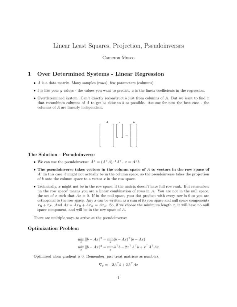
• Overdetermined system. Can’t exactly reconstruct b just from columns of A. But we want to find x
that recombines columns of A to get as close to b as possible. Assume for now the best case - the
columns of A are linearly independent.

 x 







  



=









A
b
The Solution - Pseudoinverse
• We can use the pseudoinverse: A+ = (A> A)−1 A> . x = A+ b.
• The pseudoinverse takes vectors in the column space of A to vectors in the row space of
A. In this case, b might not actually be in the column space, so the pseudoinverse takes the projection
of b onto the column space to a vector x in the row space.
• Technically, x might not be in the row space, if the matrix doesn’t have full row rank. But remember:
‘in the row space’ means you are a linear combination of rows in A. You are not in the null space,
the set of x such that Ax = 0. If in the null space, your dot product with every row is 0 so you are
orthogonal to the row space. Any x can be written as a sum of its row space and null space components
xR + xN . And Ax = AxR + AxN = AxR . So, if we choose the minimum length x, it will have no null
space component, and will be in the row space of A.
There are multiple ways to arrive at the pseudoinverse:
Optimization Problem
min kb − Axk2 = min(b − Ax)> (b − Ax)
x
x
min kb − Axk = min b> b − 2x> A> b + x> A> Ax
2
x
x
Optimized when gradient is 0. Remember, just treat matrices as numbers:
∇x = −2A> b + 2A> Ax
1
So need:
∇x = 0 = −2A> b + 2A> Ax
2A> b = 2A> Ax
A> b = A> Ax
This is called the normal equations. And is solved with
x = (A> A)−1 A> b
{z
}
|
A+
Projection Onto Column Space
• Just project b onto the column space of A to get bc and then solve Ax = bc .
• Get b’s similarity to each column vector by dotting it with each: A> b.
• Normalize weights by multiplying by (A> A)−1 . So weight vector becomes: (A> A)−1 A> b. Intuitively
you can see how this works by thinking about the case when b is a column vector. b = ci . Then we
want our weights vector to be ei . (A> A)−1 AT A = I so (A> A)−1 AT ci is just the ith column of I, aka
ei .
• Now actually use these weights to combine the columns of A to get bc . bc = A ∗ [(A> A)−1 A> b] =
A(A> A)−1 A> b
• Now we can actually solve:
Ax = bc
Ax = A(A> A)−1 A> b
x = (A> A)−1 A> b
|
{z
}
A+
Singular Value Decomposition
• Decompose A = U DV >
A
U
D
V











 
 
=
 
 







• This is the ‘truncated SVD. In general U is m × m (m is height of A), and D is m × n. But since
we have rank of A at most n, the n + 1...m columns of u are just zero columns, and only the first n
diagonal entries of D are nonzero.
Ax = b
U DV > x = b
(V D−1 U > )(U DV > )x = (V D−1 U > )b
x = (V D−1 U > )b
2
since U and V are both orthogonal matrices.
• What exactly is (V D−1 U T )? Well try the pseudoinverse:
(A> A)−1 A> = (V DU > U DV > )−1 (V DU > )
(A> A)−1 A> = (V D−2 V > )(V DU > )
(A> A)−1 A> = V D −1 U >
2
Under Determined Systems
• If A is short and fat or if A is tall but does not have full column rank. Then there are multiple x’s
such that Ax = b or that achieve min kb − Axk2 .
• Then we want to solve for the x minimizing kxk2 . And yay. The pseudoinverse gives us exactly that
x.
Optimization with Lagrange Multipliers
• Take the simplest case first and the analog to linear regression - A is short and fat but has full row
rank. Use Lagrange multiplier to optimize.
min
kxk2
x∈{x:Ax=b}
min max kxk2 + λ> (b − Ax)
x
λ
Need to have ∇x = 2x − A> λ = 0 and ∇λ = b − Ax = 0 so x = A> λ/2
0 = b − AA> λ/2
λ = 2(AA> )−1 b
so:
x = A> (AA> )−1 b
{z
}
|
A+
Projection Onto Row Space
• We want a solution x in the row space of A. So simply right x as a combination of row vectors:
x = A> w.
Ax = b
T
A(A w) = b
w = (AA> )−1 b
x = A> w = A> (AA> )−1 b
3
Under And Over Determined Systems - The Golden Goose
• A has neither full row rank nor full column rank. There is no exact solution to Ax = b, but there are
many optimal solutions.
3
• Project b onto col(A): A = U DV > , where U provides an orthonormal basis for the column space
of A. So just project b onto columns of U . bP = U w, where we can find the weights by dotting b
with each of the columns of U . So w = U > b. Since U is orthonormal, no need to normalize weights
- (U > U )−1 = I. (Remember, U is always tall and thin, or at best square, since we truncate it to
only have rank(A) columns. And since U has full column rank, U > U = I. So we now want to solve:
Ax = U U > b.
• Take x in rowspace of A: To minimize the norm of x choose an x such that x = A> c.
• Solve the new system using SVDs: Remember we are using the truncated SVD. D has all positive
diagonal entries so can be inverted, U is full column rank, and V is full row rank.
A(A> c) = U U > b
U DV > V DU > c = U U > b
U D2 U > c = U U > b
c = (U D−2 U > )U U > b
c = U D−2 U b
x = (V DU > )U D−2 U b
−1
x=V
| D{z U} b
A+
4