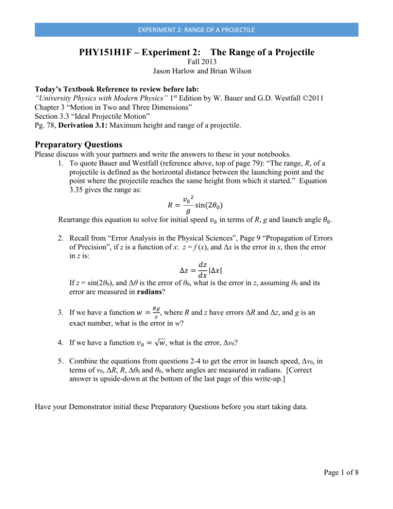
EXPERIMENT 2: RANGE OF A PROJECTILE
PHY151H1F – Experiment 2: The Range of a Projectile
Fall 2013
Jason Harlow and Brian Wilson
Today’s Textbook Reference to review before lab:
“University Physics with Modern Physics” 1st Edition by W. Bauer and G.D. Westfall ©2011
Chapter 3 “Motion in Two and Three Dimensions”
Section 3.3 “Ideal Projectile Motion”
Pg. 78, Derivation 3.1: Maximum height and range of a projectile.
Preparatory Questions
Please discuss with your partners and write the answers to these in your notebooks.
1. To quote Bauer and Westfall (reference above, top of page 79): “The range, R, of a
projectile is defined as the horizontal distance between the launching point and the
point where the projectile reaches the same height from which it started.” Equation
3.35 gives the range as:
𝑣0 2
𝑅=
sin⁡(2𝜃0 )
𝑔
Rearrange this equation to solve for initial speed 𝑣0 in terms of R, g and launch angle 𝜃0 .
2. Recall from “Error Analysis in the Physical Sciences”, Page 9 “Propagation of Errors
of Precision”, if z is a function of x: z = f (x), and Δx is the error in x, then the error
in z is:
𝑑𝑧
|∆𝑥|
∆𝑧 =
𝑑𝑥
If z = sin(2θ0), and Δθ is the error of θ0, what is the error in z, assuming θ0 and its
error are measured in radians?
𝑅𝑔
3. If we have a function 𝑤 = 𝑧 , where R and z have errors ΔR and Δz, and g is an
exact number, what is the error in w?
4. If we have a function 𝑣0 = √𝑤, what is the error, Δv0?
5. Combine the equations from questions 2-4 to get the error in launch speed, Δv0, in
terms of v0, ΔR, R, Δθ0 and θ0, where angles are measured in radians. [Correct
answer is upside-down at the bottom of the last page of this write-up.]
Have your Demonstrator initial these Preparatory Questions before you start taking data.
Page 1 of 8
EXPERIMENT 2: RANGE OF A PROJECTILE
Setting Up and Getting Started
You wish to launch a white plastic ball and investigate its range as a projectile. Figure 1 gives a
schematic of the setup.
Figure 1. Schematic of the flight of the marble over the table. The first bounce should be on
the carbon paper, which should be taped on top of a blank piece of white paper.
To launch the marble we have constructed an aluminum block which can be attached to a
PASCO cart launcher (shown in Figure 2). [NOTE: October 2013 was the first time this
apparatus has been used, so students be aware you may be “beta-testers” of this set-up!] The
launch angle can be adjusted by using the various mounting screws, to a minimum of about
5° above horizontal, and a maximum of about 85°. Once the cart launcher is set at a certain
angle, its height and position should be set so that the initial position of the bottom of the ball
when it leaves the launcher is level with the table. All of the clamps holding the cart launcher
to its stand should be fairly tight.
Figure 2. PASCO Cart Launcher Model ME-9488. From
http://www.pasco.com/prodCatalog/ME/ME-9488_cart-launcher/ .
The initial speed of the ball 𝑣0 can be adjusted by changing the amount the spring is
compressed. The amount of compression, xspring, is increased by moving the Adjustable
Latching Clamp closer to the rubber end of the shaft. The thumb screw is loosened to allow
the clamp to move and it must be tight to hold in place when the launcher is cocked. To
cock the launcher, pull back on the clamp thumb screw until the trigger is engaged on the
clamp. Then pull the string on the trigger to launch.
Page 2 of 8
EXPERIMENT 2: RANGE OF A PROJECTILE
Once you have chosen a launch angle θ and a spring compression xspring, try a few test flights
to see how far the ball goes before the first bounce. It should land on the table. Be sure to
appoint a catcher to catch the ball, because if it hits the floor it can roll a long way! When you
know where it will land, tape the carbon paper with a piece of blank paper underneath it to
the table, centered on where you think the ball will land. Then launch the ball several times.
If you launch the ball 20 times, then you expect about 68% of the landings, or about 14, to
land within the “error ellipse”, as shown in Figure 3. The range, R, is the distance from the
initial position of the ball to the centre of the error ellipse you have drawn. Half the width of
the error ellipse, along the direction of motion of the marble, is an estimate of the error in R.
Each time you change the experiment you must use a new piece of white paper, but the
carbon paper may be reused many times.
Figure 3. Example of a piece of paper after 20 hits from marble launches. An error ellipse
has been drawn so that the centre is approximately at the centre of the group of dots, and the
large and small widths have been adjusted so that approximately 68% of the dots fall within
the ellipse.
You should include at least one example of the white paper-scatter plot, along with the error
ellipse you drew, in your notebook.
The launch angle θ0 can be estimated by using the Digital Angle Gauge, and holding it
against the top of the cart launcher. Be sure to zero the gauge on a flat surface before use.
The reading error on the gauge is 0.05°. However, due to shaking of the apparatus during
launch, and the details of how the ball is launched when struck by the plunger of the cart
launcher, this measurement of the angle of the cart launcher is only a rough estimate of the
actual launch angle θ0. Jason Harlow made many measurements and determined that the
uncertainty in the launch angle when measured in this way is about Δθ0 = 3°. With a better
mounting system, this could be substantially reduced.
Page 3 of 8
EXPERIMENT 2: RANGE OF A PROJECTILE
Part A: Initial speed as a function of xspring
For a fixed value of θ (ie, θ = 30°), make a range measurement for at least 4 different
values of xspring. From your measurement of Range, (R ± ΔR), and launch angle, (θ0 ± Δθ0),
compute the initial speed of the ball v0, and its error. You may assume that g = 9.80 m/s2,
and that the error in g is small compared to your other errors.
Use PolynomialFit to make a graph of v0 (dependent variable) versus xspring (independent
variable), and fit a polynomial to this graph. Is a straight-line fit a “good” fit? Is it still a
good fit if you force the straight line to pass through the origin (xspring,v0) = (0,0)?
Part B: Initial speed as a function of θ
For a fixed value of xspring, make a range measurement for at least 4 different values of θ0.
From your measurement of Range, (R ± ΔR), and launch angle, (θ0 ± Δθ0), compute the
initial speed of the ball v0, and its error. You may assume that g = 9.80 m/s2, and that the
error in g is small compared to your other errors.
Use PolynomialFit to make a graph of v0 (dependent variable) versus θ0 (independent
variable), and fit a polynomial to this graph. In theory, we do not expect v0 to depend on
θ0. Therefore, a horizontal straight line fit of a0 only, with a1 = 0, should be a good fit. Is
a horizontal straight-line fit a “good” fit? If not, introduce other powers to your fit to make
it good. What could this mean, physically?
Additional Considerations on Experiment 2 (If You Have Time):
1) Is air resistance during the flight important?
Air resistance is discussed in Chapter 4, Section 4.7, page 121 of Bauer and Westfall. The equation is:
1
𝐹drag = 𝑐𝑑 𝐴𝜌𝑣 2
2
Here ρ = 1.2 kg/m3 is the density of the air, and for a smooth sphere you may assume that the drag
coefficient is about cd = 0.5. Input the maximum speed v you found from your range measurements, and
the cross-sectional area A of the ball, as computed from a measurement of its diameter. What is the
approximate maximum drag force Fdrag on the ball? Compare this to the force of gravity on the ball, mg.
(You will need to measure the mass of the ball using the scale which is in MP126.) If the maximum
drag force is more than 10% of the force of gravity, then air resistance is clearly important in the flight
path, and the assumption of ideal projectile motion is not valid. [Some numerical answers are upside
down on the last page of this write-up.]
2) How should v0 vary with xspring?
In Part A you measured v0 as a function of xspring. Theoretically, what do you expect for this
function? If all of the spring potential energy is converted to kinetic energy of the ball, we
might expect Us = K, where K is given by Equation 5.1: K = ½ mv2, and Us is given by
Equation 6.13: Us = ½ k x2. A more realistic model might add an “energy loss” term due to
Page 4 of 8
EXPERIMENT 2: RANGE OF A PROJECTILE
shaking of the apparatus, etc, Uloss, so that Us = K + Uloss. And an even more realistic model
might include work done by dissipative forces as the spring moves through the distance
xspring, Wloss = Fdiss xspring, so that Us = K + Uloss + Fdiss xspring. Can you redo the fits to the data
from Part A to include some of these terms?
3) What if uncertainty in the launch angle does not follow a normal distribution?
When the ball is launched, the entire cart-launcher apparatus shakes considerably. This may
introduce both a random and systematic uncertainty in our knowledge of the launch angle.
Discuss how this could affect your measurements. What if all of your measurement of angle
of the cart-launcher is systematically different from the true angle of the ball’s initial velocity
by some angle θoffset? How would it affect your Part B results if θoffset = +2°? What if θoffset
= −2°?
Create Dataset, View Dataset, and PolynomialFit are programs written in Labview by David
M. Harrison in 2007, and they are all available on the computers in MP126. They are
extremely useful programs for entering data with errors and performing proper fits using chisquared minimization.
Create Dataset Program
This program allows you to enter a dataset by hand and save it into a file. The file is tab
separated text, so may be edited with a spreadsheet program. The first row of the file contains
the title of the dataset, and the second row the names of the variables; the remaining rows are
the data, one datapoint per line.


Dataset Title: You need to give the dataset a title. We strongly recommend that you
make the title as descriptive as possible. Do NOT enter a title with a newline in it (by
pressing the Enter key).
Number of Variables: This control allows you to set the number of variables in the
dataset. Other programs (View Dataset and Polynomial Fit) assume that the data
appear in a specific order depending on the number of the variables.
Number
of
Variables
Variables
Short
Form
1
var1: the name and values of the dependent (y) variable
The value of the independent (x) variable is assumed to be 1, 2, 3, ...
y
2
var1: the name and values of the independent (x) variable
var2: the name and values of the dependent (y) variable
xy
3
var1: the name and values of the independent (x) variable
var2: the name and values of the dependent (y) variable
var3: the name and values of the error in the dependent variable
(erry)
x y erry
Page 5 of 8
EXPERIMENT 2: RANGE OF A PROJECTILE
4







var1: the name and values of the independent (x) variable
var 2 the name and values of the error in the independent variable
(errx)
var 3: the name and values of the dependent (y) variable
var 4: the name and values of the error in the dependent variable (erry)
x errx y erry
You may use the Tab key to cycle through the fields.
We recommend that you choose names for the variables that are descriptive. (ie, good variable
name: voltage [V]; poor variable name: y)
Do NOT enter a name with a newline in it (by pressing the Enter key).
Any of the following forms are equivalent: 1234.56, 1.23456E3
To completely remove a value, right click on it and choose Delete Element from the popup
menu.
The Stop button stops the program without exporting your data.
The Export button exports the dataset into a file whose name you will choose. This button is only
active when:
o Variable names have been assigned to all the variables.
o At least one datapoint has been entered.
o The number of values entered is the same for all the variables you are defining.
View Dataset Program
The program views datasets created by Create Dataset.
When the program first starts you choose the dataset file whose contents you wish to view. The display
includes:
 The title of the dataset
 The name of the datafile being shown.
 The total number of datapoints in the dataset.
 A plot of the dataset
 A table of the data in the dataset.
The table of the data includes:
 First row: a description of what the variable is.
 Second row: the name of the variable as defined in the datafile.
 Subsequent rows: the values.
You may choose to view another dataset by clicking on the Choose Another File button. The plot of
the data chooses a default way of displaying the data which is usually appropriate. The type of display
may be changed by right clicking on the Data tab in the upper-right corner of the plot, choosing
Common Plots, and selecting another type of display.
 Clicking on the Stop button exits the program
PolynomialFit Program
This program fits datasets to polynomials. Calling the independent variable x and the dependent
variable y, then the program fits to:
Page 6 of 8
EXPERIMENT 2: RANGE OF A PROJECTILE
9
𝑦 = ∑ 𝑎𝑖 𝑥 𝑖 = 𝑎0 + 𝑎1 𝑥 + 𝑎2 𝑥 2 + ⋯
𝑖=0
The program determines the values and errors of the fit coefficients ai. Controls allow you to choose
which powers of the polynomial you wish to include in the fit. The dataset is in a file that either you or
some other program has created.
 When the program starts you will be prompted to choose the file that contains the dataset to
which you wish to fit.
 The variables defined in the dataset will then be displayed in the Fit Variables part of the screen.
 You choose the terms of the polynomial by clicking on the buttons labeled with Choose the
Powers for the Fit, located near the bottom of the window. Usually these buttons are the only
things that you will need to change to fit your data to a polynomial.
 As you choose powers, the polynomial you are fitting is shown below the buttons that choose the
powers.
 When the program starts, Powers 0 and 1 are turned on, and all others are turned off. This is a fit
to a straight line: 𝑦 = 𝑎1 𝑥 + 𝑎0 . Any checked coefficients are fit, and any unchecked coefficients
are forced to be zero. For example, if only Power 1 is turned on, this fits a straight line with the
intercept forced to zero. Only the slope a1 is fit.
 You may change the powers at any time and the results of the new fit will be displayed. The
most important of these results are:
o Fit Coefficients: Value ± Error. This is a table of the values of the fit coefficients and
their estimated errors.
o Residuals plot. The residuals are the values of the dependent (y) variables as given by the
fit minus the values in the dataset. For a good fit the residuals should be small and
randomly distributed around zero. If this is not the case either there is something wrong
with the data or you are trying to fit the data to an incorrect model.
o Fit Result Plot. This shows the data and the results of the fit.
 Adjust Significant Figures: By default the fitter adjusts the values of the parameter values
based on their errors. This makes the values easier to read. Clicking on the Adjust Sig Figs
switch allows you to turn this adjustment off; clicking on it again turns the adjustment back on.
These adjusted values are what is used in displaying the Fit Result in the graph. Occasionally
rounding errors can cause the resulting graph to look silly. Sometimes turning off the adjustment
fixes this.
 Reweight: If the data do not have explicit errors, by default the data are weighted by assigning
an error in the dependent (y) variable equal to the square root of (sum of the squares / degrees of
freedom). This does not affect the values of the fit coefficients, but does usually make the
estimates of their errors more realistic. Clicking on the Reweight switch allows you to turn off
this reweighting and have the fitter assume that there are no errors in the dependent variable;
clicking on the switch again turns reweighting back on. For most experimental data, reweighting
is the right thing to do.
 Evaluating the Fit: As already mentioned, if the data are good and the model being fit to is
appropriate then the residuals should be small and randomly distributed around zero. Here are a
couple of tips for determining the best fit to the data.
Page 7 of 8
EXPERIMENT 2: RANGE OF A PROJECTILE

1. If the value of a parameter is zero within errors, remove that power from the fit.
2. Even if the value of a parameter is not zero within errors, if removing that power from the fit
does not make any appreciable difference in the Fit Result Plot you may wish to consider
leaving the power out of the fit.
Chi-Squared: If there are explicit errors in one or both coordinates of the dataset then the ChiSquared is shown. This is related to the sum of the squares of the residuals, except that the data
are weighted with the explicit errors. To interpret the chi-squared one needs to also look at the
Degrees of Freedom of the fit, whose value is also shown. This number is the number of
datapoints in the data minus the number of parameters to which you are fitting. The rules are:
o If the Chi-Squared is much greater than the Degrees of Freedom, then the fit is poor.
o If the Chi-Squared is much less than the Degrees of Freedom, then the fit is “too good to
be true”, and is suspect. A common cause of this behavior is when the explicit errors are
larger than is appropriate.
o The best result is when the Chi-Squared is approximately equal to the Degrees of
Freedom.
Page 8 of 8