Robust Image Sentiment Analysis Using Progressively Trained and Domain
Transferred Deep Networks
Quanzeng You and Jiebo Luo
Hailin Jin and Jianchao Yang
Department of Computer Science
University of Rochester
Rochester, NY 14623
{qyou, jluo}@cs.rochester.edu
Adobe Research
345 Park Avenue
San Jose, CA 95110
{hljin, jiayang}@adobe.com
Abstract
Sentiment analysis of online user generated content is
important for many social media analytics tasks. Researchers have largely relied on textual sentiment analysis to develop systems to predict political elections, measure economic indicators, and so on. Recently,
social media users are increasingly using images and
videos to express their opinions and share their experiences. Sentiment analysis of such large scale visual
content can help better extract user sentiments toward
events or topics, such as those in image tweets, so that
prediction of sentiment from visual content is complementary to textual sentiment analysis. Motivated by the
needs in leveraging large scale yet noisy training data to
solve the extremely challenging problem of image sentiment analysis, we employ Convolutional Neural Networks (CNN). We first design a suitable CNN architecture for image sentiment analysis. We obtain half a
million training samples by using a baseline sentiment
algorithm to label Flickr images. To make use of such
noisy machine labeled data, we employ a progressive strategy to fine-tune the deep network. Furthermore, we
improve the performance on Twitter images by inducing domain transfer with a small number of manually
labeled Twitter images. We have conducted extensive
experiments on manually labeled Twitter images. The
results show that the proposed CNN can achieve better
performance in image sentiment analysis than competing algorithms.
Introduction
Online social networks are providing more and more convenient services to their users. Today, social networks have
grown to be one of the most important sources for people to
acquire information on all aspects of their lives. Meanwhile,
every online social network user is a contributor to such
large amounts of information. Online users love to share
their experiences and to express their opinions on virtually
all events and subjects.
Among the large amount of online user generated data, we
are particularly interested in people’s opinions or sentiments
towards specific topics and events. There have been many
c 2015, Association for the Advancement of Artificial
Copyright Intelligence (www.aaai.org). All rights reserved.
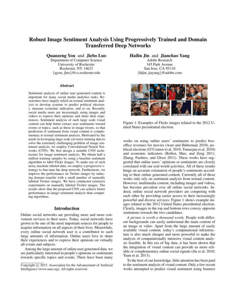
Figure 1: Examples of Flickr images related to the 2012 United States presidential election.
works on using online users’ sentiments to predict boxoffice revenues for movies (Asur and Huberman 2010), political elections (O’Connor et al. 2010; Tumasjan et al. 2010)
and economic indicators (Bollen, Mao, and Zeng 2011;
Zhang, Fuehres, and Gloor 2011). These works have suggested that online users’ opinions or sentiments are closely
correlated with our real-world activities. All of these results
hinge on accurate estimation of people’s sentiments according to their online generated content. Currently all of these
works only rely on sentiment analysis from textual content.
However, multimedia content, including images and videos,
has become prevalent over all online social networks. Indeed, online social network providers are competing with
each other by providing easier access to their increasingly
powerful and diverse services. Figure 1 shows example images related to the 2012 United States presidential election.
Clearly, images in the top and bottom rows convey opposite
sentiments towards the two candidates.
A picture is worth a thousand words. People with different backgrounds can easily understand the main content of
an image or video. Apart from the large amount of easily
available visual content, today’s computational infrastructure is also much cheaper and more powerful to make the
analysis of computationally intensive visual content analysis feasible. In this era of big data, it has been shown that
the integration of visual content can provide us more reliable or complementary online social signals (Jin et al. 2010;
Yuan et al. 2013).
To the best of our knowledge, little attention has been paid
to the sentiment analysis of visual content. Only a few recent
works attempted to predict visual sentiment using features
from images (Siersdorfer et al. 2010; Borth et al. 2013b;
2013a; Yuan et al. 2013) and videos (Morency, Mihalcea,
and Doshi 2011). Visual sentiment analysis is extremely
challenging. First, image sentiment analysis is inherently
more challenging than object recognition as the latter is usually well defined. Image sentiment involves a much higher
level of abstraction and subjectivity in the human recognition process (Joshi et al. 2011), on top of a wide variety of
visual recognition tasks including object, scene, action and
event recognition. In order to use supervised learning, it is
imperative to collect a large and diverse labeled training set
perhaps on the order of millions of images. This is an almost
insurmountable hurdle due to the tremendous labor required
for image labeling. Second, the learning schemes need to
have high generalizability to cover more different domains.
However, the existing works use either pixel-level features
or a limited number of predefined attribute features, which
is difficult to adapt the trained models to images from a different domain.
The deep learning framework enables robust and accurate
feature learning, which in turn produces the state-of-the-art
performance on digit recognition (LeCun et al. 1989; Hinton, Osindero, and Teh 2006), image classification (Cireşan
et al. 2011; Krizhevsky, Sutskever, and Hinton 2012), musical signal processing (Hamel and Eck 2010) and natural
language processing (Maas et al. 2011). Both the academia
and industry have invested a huge amount of effort in building powerful neural networks. These works suggested that
deep learning is very effective in learning robust features in a
supervised or unsupervised fashion. Even though deep neural networks may be trapped in local optima (Hinton 2010;
Bengio 2012), using different optimization techniques, one
can achieve the state-of-the-art performance on many challenging tasks mentioned above.
Inspired by the recent successes of deep learning, we are
interested in solving the challenging visual sentiment analysis task using deep learning algorithms. For images related tasks, Convolutional Neural Network (CNN) are widely
used due to the usage of convolutional layers. It takes into
consideration the locations and neighbors of image pixels, which are important to capture useful features for visual
tasks. Convolutional Neural Networks (LeCun et al. 1998;
Cireşan et al. 2011; Krizhevsky, Sutskever, and Hinton
2012) have been proved very powerful in solving computer
vision related tasks. We intend to find out whether applying
CNN to visual sentiment analysis provides advantages over
using a predefined collection of low-level visual features or
visual attributes, which have been done in prior works.
To that end, we address in this work two major challenges:
1) how to learn with large scale weakly labeled training data, and 2) how to generalize and extend the learned model
across domains. In particular, we make the following contributions.
• We develop an effective deep convolutional network architecture for visual sentiment analysis. Our architecture
employs two convolutional layers and several fully connected layers for the prediction of visual sentiment labels.
• Our model attempts to address the weakly labeled nature
of the training image data, where such labels are machine
generated, by leveraging a progressive training strategy
and a domain transfer strategy to fine-tune the neural network. Our evaluation results suggest that this strategy is
effective for improving the performance of neural network in terms of generalizability.
• In order to evaluate our model as well as competing algorithms, we build a large manually labeled visual sentiment
dataset using Amazon Mechanical Turk. This dataset will
be released to the research community to promote further
investigations on visual sentiment.
Related Work
In this section, we review literature closely related to our
study on visual sentiment analysis, particularly in sentiment
analysis and Convolutional Neural Networks.
Sentiment Analysis
Sentiment analysis is a very challenging task (Liu et al.
2003; Li et al. 2010). Researchers from natural language
processing and information retrieval have developed different approaches to solve this problem, achieving promising
or satisfying results (Pang and Lee 2008). In the context of
social media, there are several additional unique challenges.
First, there are huge amounts of data available. Second, messages on social networks are by nature informal and short.
Third, people use not only textual messages, but also images
and videos to express themselves.
Tumasjan et al. (2010) and Bollen et al. (2011) employed
pre-defined dictionaries for measuring the sentiment level
of Tweets. The volume or percentage of sentiment-bearing
words can produce an estimate of the sentiment of one particular tweet. Davidov et al. (2010) used the weak labels
from a large amount of Tweets. In contrast, they manually selected hashtags with strong positive and negative sentiments and ASCII smileys are also utilized to label the sentiments of tweets. Furthermore, Hu et al. (2013) incorporated social signals into their unsupervised sentiment analysis
framework. They defined and integrated both emotion indication and correlation into a framework to learn parameters
for their sentiment classifier.
There are also several recent works on visual sentiment
analysis. Siersdorfer et al. (2010) proposes a machine learning algorithm to predict the sentiment of images using pixellevel features. Motivated by the fact that sentiment involves
high-level abstraction, which may be easier to explain by
objects or attributes in images, both (Borth et al. 2013a)
and (Yuan et al. 2013) propose to employ visual entities or
attributes as features for visual sentiment analysis. In (Borth
et al. 2013a), 1200 adjective noun pairs (ANP), which may
correspond to different levels of different emotions, are extracted. These ANPs are used as queries to crawl images
from Flickr. Next, pixel-level features of images in each ANP are employed to train 1200 ANP detectors. The responses
of these 1200 classifiers can then be considered as mid-level
features for visual sentiment analysis. The work in (Yuan et
al. 2013) employed a similar mechanism. The main difference is that 102 scene attributes are used instead.
256
11
11
227
227
5
5
27
2
55
227
27
55
227
3
96
24
256
512
512
256
3
Figure 2: Convolutional Neural Network for Visual Sentiment Analysis.
Convolutional Neural Networks
Convolutional Neural Networks (CNN) have been very successful in document recognition (LeCun et al. 1998). CNN
typically consists of several convolutional layers and several fully connected layers. Between the convolutional layers,
there may also be pooling layers and normalization layers.
CNN is a supervised learning algorithm, where parameters of different layers are learned through back-propagation.
Due to the computational complexity of CNN, it has only be
applied to relatively small images in the literature. Recently,
thanks to the increasing computational power of GPU, it is
now possible to train a deep convolutional neural network on
a large scale image dataset (Krizhevsky, Sutskever, and Hinton 2012). Indeed, in the past several years, CNN has been
successfully applied to scene parsing (Grangier, Bottou, and
Collobert 2009), feature learning (LeCun, Kavukcuoglu, and
Farabet 2010), visual recognition (Kavukcuoglu et al. 2010)
and image classification (Krizhevsky, Sutskever, and Hinton
2012). In our work, we intend to use CNN to learn features
which are useful for visual sentiment analysis.
Visual Sentiment Analysis
We propose to develop a suitable convolutional neural network architecture for visual sentiment analysis. Moreover,
we employ a progressive training strategy that leverages the
training results of convolutional neural network to further
filter out (noisy) training data. The details of the proposed
framework will be described in the following sections.
Visual Sentiment Analysis with regular CNN
CNN has been proven to be effective in image classification tasks, e.g., achieving the state-of-the-art performance
in ImageNet Challenge (Krizhevsky, Sutskever, and Hinton
2012). Visual sentiment analysis can also be treated as an
image classification problem. It may seem to be a much
easier problem than image classification from ImageNet (2
classes vs. 1000 classes in ImageNet). However, visual sentiment analysis is quite challenging because sentiments or
opinions correspond to high level abstractions from a given image. This type of high level abstraction may require
viewer’s knowledge beyond the image content itself. Meanwhile, images in the same class of ImageNet mainly contain
the same type of object. In sentiment analysis, each class
contains much more diverse images. It is therefore extremely challenging to discover features which can distinguish
much more diverse classes from each other. In addition, people may have totally different sentiments over the same image. This adds difficulties to not only our classification task,
but also the acquisition of labeled images. In other words, it is nontrivial to obtain highly reliable labeled instances,
let alone a large number of them. Therefore, we need a supervised learning engine that is able to tolerate a significant
level of noise in the training dataset.
The architecture of the CNN we employ for sentiment analysis is shown in Figure 2. Each image is resized to
256 × 256 (if needed, we employ center crop, which first
resizes the shorter dimension to 256 and then crops the middle section of the resized image). The resized images are
processed by two convolutional layers. Each convolutional
layer is also followed by max-pooling layers and normalization layers. The first convolutional layer has 96 kernels of
size 11 × 11 × 3 with a stride of 4 pixels. The second convolutional layer has 256 kernels of size 5 × 5 with a stride
of 2 pixels. Furthermore, we have four fully connected layers. Inspired by (Çaglar Gülçehre et al. 2013), we constrain
the second to last fully connected layer to have 24 neurons. According to the Plutchik’s wheel of emotions (Plutchik
1984), there are a total of 24 emotions belonging to two categories: positive emotions and negative emotions. Intuitively.
we hope these 24 nodes may help the network to learn the 24
emotions from a given image and then classify each image
into positive or negative class according to the responses of
these 24 emotions.
The last layer is designed to learn the parameter w by
maximizing the following conditional log likelihood function (xi and yi are the feature vector and label for the i-th
instance respectively):
l(w) =
n
X
ln p(yi = 1|xi , w) + (1 − yi ) ln p(yi = 0|xi , w)
i=1
(1)
where
p(yi |xi , w) =
exp(w0 +
Pk
1 + exp(w0 +
j=1
Pk
wj xij )yi
j=1
wj xij )yi
(2)
5) Fine-tune
1) Input
2) CNN model
...
Train convolutional Neural Network
CNN
3)
4) Sampling
Predict
f(·)
PCNN
6) PCNN model
Figure 3: Progressive CNN (PCNN) for visual sentiment analysis.
Visual Sentiment Analysis with Progressive CNN
Since the images are weakly labeled, it is possible that the
neural network can get stuck in a bad local optimum. This
may lead to poor generalizability of the trained neural network. On the other hand, we found that the neural network
is still able to correctly classify a large proportion of the
training instances. In other words, the neural network has
learned knowledge to distinguish the training instances with
relatively distinct sentiment labels. Therefore, we propose to
progressively select a subset of the training instances to reduce the impact of noisy training instances. Figure 3 shows
the overall flow of the proposed progressive CNN (PCNN). We first train a CNN on Flickr images. Next, we select training samples according to the prediction score of the
trained model on the training data itself. Instead of training
from the beginning, we further fine-tune the trained model
using these newly selected, and potentially cleaner training
instances. This fine-tuned model will be our final model for
visual sentiment analysis.
Algorithm 1 Progressive CNN training for Visual Sentiment
Analysis
Input: X = {x1 , x2 , . . . , xn } a set of images of size 256 ×
256
Y = {y1 , y2 , . . . , yn } sentiment labels of X
1: Train convolutional neural network CNN with input X
and Y
2: Let S ∈ Rn×2 be the sentiment scores of X predicted
using CNN
3: for si ∈ S do
4:
Delete xi from X with probability pi (Eqn.(3))
5: end for
6: Let X 0 ⊂ X be the remaining training images, Y 0 be
their sentiment labels
7: Fine-tune CNN with input X 0 and Y 0 to get PCNN
8: return PCNN
In particular, we employ a probabilistic sampling algorithm to select the new training subset. The intuition is that
we want to keep instances with distinct sentiment scores between the two classes with a high probability, and conversely remove instances with similar sentiment scores for both
classes with a high probability. Let si = (si1 , si2 ) be the
prediction sentiment scores for the two classes of instance i.
We choose to remove the training instance i with probability
pi given by Eqn.(3). Algorithm 1 summarizes the steps of
the proposed framework.
pi = max (0, 2 − exp(|si1 − si2 |))
(3)
When the difference between the predicted sentiment scores
of one training instance are large enough, this training instance will be kept in the training set. Otherwise, the smaller
the difference between the predicted sentiment scores become, the larger the probability of this instance being removed from the training set.
Experiments
We choose to use the same half million Flickr images
from SentiBank1 to train our Convolutional Neural Network.
These images are only weakly labeled since each image belongs to one adjective noun pair (ANP). There are a total
of 1200 ANPs. According to the Plutchik’s Wheel of Emotions (Plutchik 1984), each ANP is generated by the combination of adjectives with strong sentiment values and nouns
from tags of images and videos (Borth et al. 2013b). These
ANPs are then used as queries to collect related images
for each ANP. The released SentiBank contains 1200 ANPs
with about half million Flickr images. We train our convolutional neural network mainly on this image dataset. We implement the proposed architecture of CNN on the publicly
available implementation Caffe (Jia 2013). All of our experiments are evaluated on a Linux X86 64 machine with 32G
RAM and two NVIDIA GTX Titan GPUs.
Comparisons of different CNN architectures
The architecture of our model is shown in Figure 2. However, we also evaluate other architectures for the visual sentiment analysis task. Table 1 summarizes the performance of
different architectures on a randomly chosen Flickr testing
1
http://visual-sentiment-ontology.appspot.com/
dataset. In Table 1, iCONV-jFC indicates that there are i
convolutional layers and j fully connected layers in the architecture. The model in Figure 2 shows slightly better performance than other models in terms of F1 and accuracy. In
the following experiments, we mainly focus on the evaluation of CNN using the architecture in Figure 2.
Table 1: Summary of performance of different architectures
on randomly chosen testing data.
Architecture
3CONV-4FC
3CONV-2FC
2CONV-3FC
2CONV-4FC
Precision
0.679
0.69
0.679
0.688
Recall
0.845
0.847
0.874
0.875
F1
0.753
0.76
0.765
0.77
Accuracy
0.644
0.657
0.654
0.665
Baselines
We compare the performance of PCNN with three other
baselines or competing algorithms for image sentiment classification.
Low-level Feature-based Siersdorfer et al. (2010) defined
both global and local visual features. Specifically, the global color histograms (GCH) features consist of 64-bin RGB
histogram. The local color histogram features (LCH) first
divided the image into 16 blocks and used the 64-bin RGB
histogram for each block. They also employed SIFT features
to learn a visual word dictionary. Next, they defined bag of
visual word features (BoW) for each image.
Mid-level Feature-based Damian et al. (2013a; 2013b)
proposed a framework to build visual sentiment ontology
and SentiBank according to the previously discussed 1200
ANPs. With the trained 1200 ANP detectors, they are able
to generate 1200 responses for any given test image using
these pre-trained 1200 ANP detectors. A sentiment classifier is built on top of these mid-level features according to the
sentiment label of training images. Sentribute (Yuan et al.
2013) also employed mid-level features for sentiment prediction. However, instead of using adjective noun pairs, they
employed scene-based attributes (Patterson and Hays 2012)
to define the mid-level features.
Deep Learning on Flickr Dataset
We randomly choose 90% images from the half million
Flickr images as our training dataset. The remaining 10%
images are our testing dataset. We train the convolutional neural network with 300,000 iterations of mini-batches
(each mini-batch contains 256 images). We employ the sampling probability in Eqn.(3) to filter the training images according to the prediction score of CNN on its training data.
In the fine-tuning stage of PCNN, we run another 100,000
iterations of mini-batches using the filtered training dataset.
Table 2 gives a summary of the number of data instances in
our experiments. Figure 4 shows the filters learned in the
first convolutional layer of CNN and PCNN, respectively.
There are some differences between 4(a) and 4(b). While
it is somewhat inconclusive that the neural networks have
reached a better local optimum, at least we can conclude that
Table 2: Statistics of the number of Flickr image dataset.
Models training testing # of iterations
CNN
401,739 44,637
300,000
PCNN
369,828 44,637
100,000
Table 3: Performance on the Testing Dataset by CNN and
PCNN.
Algorithm
CNN
PCNN
Precision
0.714
0.759
Recall
0.729
0.826
F1
0.722
0.791
Accuracy
0.718
0.781
the fine-tuning stage using a progressively cleaner training
dataset has prompted the neural networks to learn different
knowledge. Indeed, the evaluation results suggest that this
fine-tuning leads to the improvement of performance.
Table 3 shows the performance of both CNN and PCNN
on the 10% randomly chosen testing data. PCNN outperformed CNN in terms of Precision, Recall, F1 and Accuracy. The results in Table 3 and the filters from Figure 4 shows
that the fine-tuning stage of PCNN can help the neural network to search for a better local optimum.
(a) Filters learned from CNN
(b) Filters learned from PCNN
Figure 4: Filters of the first convolutional layer.
Twitter Testing Dataset
We also built a new image dataset from image tweets. Image tweets refer to those tweets that contain images. We
built a total of 1269 images as our candidate testing images.
We employed crowd intelligence, Amazon Mechanical Turk
(AMT), to generate sentiment labels for these testing images, in a similar fashion to (Borth et al. 2013b). We recruited 5 AMT workers for each of the candidate image. Table 4
shows the statistics of the labeling results from the Amazon
Mechanical Turk. In the table, “five agree” indicates that all the 5 AMT workers gave the same sentiment label for a
given image. Only a small portion of the images, 153 out of
1269, had significant disagreements between the 5 worker-
Table 5: Performance of different algorithms on the Twitter image dataset (Acc stands for Accuracy).
Algorithms
CNN
PCNN
Precision
0.749
0.77
Five Agree
Recall
F1
0.869
0.805
0.878
0.821
Acc
0.722
0.747
At Least Four Agree
Precision Recall
F1
0.707
0.839
0.768
0.733
0.845
0.785
Acc
0.686
0.714
At Least Three Agree
Precision Recall
F1
Acc
0.691
0.814
0.747 0.667
0.714
0.806
0.757 0.687
s (3 vs. 2). We evaluate the performance of ConvolutionTable 4: Summary of AMT labeled results for the Twitter
testing dataset.
Sentiment
Five Agree
Positive
Negative
Sum
581
301
882
At Least Four
Agree
689
427
1116
At Least
Three Agree
769
500
1269
al Neural Networks on this manually labeled image dataset
according to the model trained on Flickr images. Table 5
shows the performance of the two frameworks. Not surprisingly, both models perform better on the less ambiguous image set (“five agree” by AMT). Meanwhile, PCNN shows
better performance than CNN on all the three labeling sets in terms of both F1 and accuracy. This suggests that the
fine-tuning stage of CNN effectively improves the generalizability extensibility of the neural networks.
Transfer Learning
Half million Flickr images are used in our CNN training.
The features learned are generic features on these half million images. Table 5 shows that these generic features also
have the ability to predict visual sentiment of images from
other domains. The question we ask is whether we can further improve the performance of visual sentiment analysis
on Twitter images by inducing transfer learning. In this section, we conduct experiments to answer this question.
The users of Flickr are more likely to spend more time
on taking high quality pictures. Twitter users are likely to
share the moment with the world. Thus, most of the Twitter
images are casually taken snapshots. Meanwhile, most of the
images are related to current trending topics and personal
experiences, making the images on Twitter much diverse in
content as well as quality.
In this experiment, we fine-tune the pre-trained neural network model in the following way to achieve transfer learning. We randomly divide the Twitter images into 5 equal partitions. Every time, we use 4 of the 5 partitions to fine-tune
our pre-trained model from the half million Flickr images
and evaluate the new model on the remaining partition. The
averaged evaluation results are reported. The algorithm is
detailed in Algorithm 2.
Similar to (Borth et al. 2013b), we also employ 5-fold
cross-validation to evaluate the performance of all the baseline algorithms. Table 6 summarizes the averaged performance results of different baseline algorithms and our two
CNN models. Overall, both CNN models outperform the
baseline algorithms. In the baseline algorithms, Sentribute
Figure 5: Positive (top block) and Negative (bottom block)
examples. Each column shows the negative example images for each algorithm (PCNN, CNN, Sentribute, Sentibank, GCH, LCH, GCH+BoW, LCH+BoW). The images
are ranked by the prediction score from top to bottom in a
decreasing order.
Algorithm 2 Transfer Learning to fine-tune CNN
Input: X = {x1 , x2 , . . . , xn } a set of images of size 256 ×
256
Y = {y1 , y2 , . . . , yn } sentiment labels of X
Pre-trained CNN model M
1: Randomly partition X and Y into 5 equal groups
{(X1 , Y1 ), . . . , (X5 , Y5 )}.
2: for i from 1 to 5 do
3:
Let (X 0 , Y 0 ) = (X, Y ) − (Xi , Yi )
4:
Fine-tune M with input (X 0 , Y 0 ) to obtain model Mi
5:
Evaluate the performance of Mi on (Xi , Yi )
6: end for
7: return The averaged performance of Mi on (Xi , Yi ) (i
from 1 to 5)
gives slightly better results than the other two baseline algorithms. Interestingly, even the combination of using low-
Table 6: 5-Fold Cross-Validation Performance of different algorithms on the Twitter image dataset. Note that compared with
Table 5, both fine-tuned CNN models have been improved due to domain transfer learning (Acc stands for Accuracy).
Algorithms
GCH
LCH
GCH + BoW
LCH + BoW
SentiBank
Sentribute
CNN
PCNN
Precision
0.708
0.764
0.724
0.771
0.785
0.789
0.795
0.797
Five Agree
Recall
F1
0.888
0.787
0.809
0.786
0.904
0.804
0.811
0.79
0.768
0.776
0.823
0.805
0.905
0.846
0.881
0.836
Acc
0.684
0.71
0.71
0.717
0.709
0.738
0.783
0.773
At Least Four Agree
Precision Recall
F1
0.687
0.84
0.756
0.725
0.753
0.739
0.703
0.849
0.769
0.751
0.762
0.756
0.742
0.727
0.734
0.75
0.792
0.771
0.773
0.855
0.811
0.786
0.842
0.811
level features local color histogram (LCH) and bag of visual words (BoW) shows better results than SentiBank on
our Twitter dataset. Both fine-tuned CNN models have been
improved. This improvement is significant given that we only use four fifth of the 1269 images for domain adaptation.
Both neural network models have similar performance on all
the three sets of the Twitter testing data. This suggests that
the fine-tuning stage helps both models to find a better local minimum. In particular, the knowledge from the Twitter
images starts to determine the performance of both neural
networks. The previously trained model only determines the
start position of the fine-tuned model.
Meanwhile, for each model, we respectively select the top
5 positive and top 5 negative examples from the 1269 Twitter images according to the evaluation scores. Figure show
those examples for each model. In both figures, each column
contains the images for one model. A green solid box means
the prediction label of the image agrees with the human label. Otherwise, we use a red dashed box. The labels of top
ranked images in both neural network models are all correctly predicted. However, the images are not all the same. This
on the other hand suggests that even though the two models
achieve similar results after fine-tuning, they may have arrived at somewhat different local optima due to the different
starting positions, as well as the transfer learning process.
For all the baseline models, it is difficult to say which kind
of images are more likely to be correctly classified according
to these images. However, we observe that there are several
mistakenly classified images in common among the models
using low-level features (the four rightmost columns in Figure ). Similarly, for Sentibank and Sentribute, several of the
same images are also in the top ranked samples. This indicates that there are some common learned knowledge in the
low-level feature models and mid-level feature models.
Conclusions
Visual sentiment analysis is a challenging and interesting
problem. In this paper, we adopt the recent developed convolutional neural networks to solve this problem. We have
designed a new architecture, as well as new training strategies to overcome the noisy nature of the large-scale training samples. Both progressive training and transfer learning
inducted by a small number of confidently labeled images
from the target domain have yielded notable improvements.
Acc
0.665
0.671
0.685
0.697
0.675
0.709
0.755
0.759
At Least Three Agree
Precision Recall
F1
0.678
0.836
0.749
0.716
0.737
0.726
0.683
0.835
0.751
0.722
0.726
0.723
0.720
0.723
0.721
0.733
0.783
0.757
0.734
0.832
0.779
0.755
0.805
0.778
Acc
0.66
0.664
0.665
0.664
0.662
0.696
0.715
0.723
The experimental results suggest that convolutional neural
networks that are properly trained can outperform both classifiers that use predefined low-level features or mid-level visual attributes for the highly challenging problem of visual
sentiment analysis. Meanwhile, the main advantage of using convolutional neural networks is that we can transfer
the knowledge to other domains using a much simpler finetuning technique than those in the literature e.g., (Duan et al.
2012).
It is important to reiterate the significance of this work
over the state-of-the-art (Siersdorfer et al. 2010; Borth et al.
2013b; Yuan et al. 2013). We are able to directly leverage a
much larger weakly labeled data set for training, as well as
a larger manually labeled dataset for testing. The larger data sets, along with the proposed deep CNN and its training
strategies, give rise to better generalizability of the trained
model and higher confidence of such generalizability. In the
future, we plan to develop robust multimodality models that
employ both the textual and visual content for social media sentiment analysis. We also hope our sentiment analysis
results can encourage further research on online user generated content.
We believe that sentiment analysis on large scale online
user generated content is quite useful since it can provide
more robust signals and information for many data analytics
tasks, such as using social media for prediction and forecasting. In the future, we plan to develop robust multimodality
models that employ both the textual and visual content for
social media sentiment analysis. We also hope our sentiment
analysis results can encourage further research on online user generated content.
Acknowledgments
This work was generously supported in part by Adobe Research. We would like to thank Digital Video and Multimedia (DVMM) Lab at Columbia University for providing the
half million Flickr images and their machine-generated labels.
References
Asur, S., and Huberman, B. A. 2010. Predicting the future
with social media. In WI-IAT, volume 1, 492–499. IEEE.
Bengio, Y. 2012. Practical recommendations for gradient-
based training of deep architectures. In Neural Networks:
Tricks of the Trade. Springer. 437–478.
Bollen, J.; Mao, H.; and Pepe, A. 2011. Modeling public
mood and emotion: Twitter sentiment and socio-economic
phenomena. In ICWSM.
Bollen, J.; Mao, H.; and Zeng, X. 2011. Twitter mood predicts the stock market. Journal of Computational Science
2(1):1–8.
Borth, D.; Chen, T.; Ji, R.; and Chang, S.-F. 2013a. Sentibank: large-scale ontology and classifiers for detecting sentiment and emotions in visual content. In ACM MM, 459–
460. ACM.
Borth, D.; Ji, R.; Chen, T.; Breuel, T.; and Chang, S.-F.
2013b. Large-scale visual sentiment ontology and detectors
using adjective noun pairs. In ACM MM, 223–232. ACM.
Çaglar Gülçehre; Cho, K.; Pascanu, R.; and Bengio, Y. 2013.
Learned-norm pooling for deep neural networks. CoRR abs/1311.1780.
Cireşan, D. C.; Meier, U.; Masci, J.; Gambardella, L. M.;
and Schmidhuber, J. 2011. Flexible, high performance convolutional neural networks for image classification. In IJCAI, 1237–1242. AAAI Press.
Davidov, D.; Tsur, O.; and Rappoport, A. 2010. Enhanced
sentiment learning using twitter hashtags and smileys. In
ICL, 241–249. Association for Computational Linguistics.
Duan, L.; Xu, D.; Tsang, I.-H.; and Luo, J. 2012. Visual
event recognition in videos by learning from web data. IEEE
PAMI 34(9):1667–1680.
Grangier, D.; Bottou, L.; and Collobert, R. 2009. Deep
convolutional networks for scene parsing. In ICML 2009
Deep Learning Workshop, volume 3. Citeseer.
Hamel, P., and Eck, D. 2010. Learning features from music
audio with deep belief networks. In ISMIR, 339–344.
Hinton, G. E.; Osindero, S.; and Teh, Y.-W. 2006. A fast
learning algorithm for deep belief nets. Neural computation
18(7):1527–1554.
Hinton, G. 2010. A practical guide to training restricted
boltzmann machines. Momentum 9(1):926.
Hu, X.; Tang, J.; Gao, H.; and Liu, H. 2013. Unsupervised
sentiment analysis with emotional signals. In WWW, 607–
618. International World Wide Web Conferences Steering
Committee.
Jia, Y. 2013. Caffe: An open source convolutional architecture for fast feature embedding. http://caffe.
berkeleyvision.org/.
Jin, X.; Gallagher, A.; Cao, L.; Luo, J.; and Han, J. 2010.
The wisdom of social multimedia: using flickr for prediction
and forecast. In ACM MM, 1235–1244. ACM.
Joshi, D.; Datta, R.; Fedorovskaya, E.; Luong, Q.-T.; Wang,
J. Z.; Li, J.; and Luo, J. 2011. Aesthetics and emotions in
images. IEEE Signal Processing Magazine 28(5):94–115.
Kavukcuoglu, K.; Sermanet, P.; Boureau, Y.-L.; Gregor, K.;
Mathieu, M.; and LeCun, Y. 2010. Learning convolutional
feature hierarchies for visual recognition. In NIPS, 5.
Krizhevsky, A.; Sutskever, I.; and Hinton, G. E. 2012. Imagenet classification with deep convolutional neural networks. In NIPS, 4.
LeCun, Y.; Boser, B.; Denker, J. S.; Henderson, D.; Howard,
R. E.; Hubbard, W.; and Jackel, L. D. 1989. Backpropagation applied to handwritten zip code recognition. Neural
computation 1(4):541–551.
LeCun, Y.; Bottou, L.; Bengio, Y.; and Haffner, P. 1998.
Gradient-based learning applied to document recognition.
Proceedings of the IEEE 86(11):2278–2324.
LeCun, Y.; Kavukcuoglu, K.; and Farabet, C. 2010. Convolutional networks and applications in vision. In ISCAS,
253–256. IEEE.
Li, G.; Hoi, S. C.; Chang, K.; and Jain, R. 2010. Microblogging sentiment detection by collaborative online learning. In ICDM, 893–898. IEEE.
Liu, B.; Dai, Y.; Li, X.; Lee, W. S.; and Yu, P. S. 2003. Building text classifiers using positive and unlabeled examples. In
ICDM, 179–186. IEEE.
Maas, A. L.; Daly, R. E.; Pham, P. T.; Huang, D.; Ng, A. Y.;
and Potts, C. 2011. Learning word vectors for sentiment
analysis. In ACL, 142–150.
Morency, L.-P.; Mihalcea, R.; and Doshi, P. 2011. Towards multimodal sentiment analysis: Harvesting opinions from
the web. In ICMI, 169–176. New York, NY, USA: ACM.
O’Connor, B.; Balasubramanyan, R.; Routledge, B. R.; and
Smith, N. A. 2010. From tweets to polls: Linking text sentiment to public opinion time series. ICWSM 11:122–129.
Pang, B., and Lee, L. 2008. Opinion mining and sentiment
analysis. Foundations and trends in information retrieval
2(1-2):1–135.
Patterson, G., and Hays, J. 2012. Sun attribute database:
Discovering, annotating, and recognizing scene attributes. In
CVPR.
Plutchik, R. 1984. Emotions: A general psychoevolutionary
theory. Approaches to emotion 1984:197–219.
Siersdorfer, S.; Minack, E.; Deng, F.; and Hare, J. 2010.
Analyzing and predicting sentiment of images on the social
web. In ACM MM, 715–718. ACM.
Tumasjan, A.; Sprenger, T. O.; Sandner, P. G.; and Welpe,
I. M. 2010. Predicting elections with twitter: What 140
characters reveal about political sentiment. ICWSM 178–
185.
Yuan, J.; Mcdonough, S.; You, Q.; and Luo, J. 2013. Sentribute: image sentiment analysis from a mid-level perspective. In Proceedings of the Second International Workshop
on Issues of Sentiment Discovery and Opinion Mining, 10.
ACM.
Zhang, X.; Fuehres, H.; and Gloor, P. A. 2011. Predicting
stock market indicators through twitter i hope it is not as bad
as i fear. Procedia-Social and Behavioral Sciences 26:55–
62.