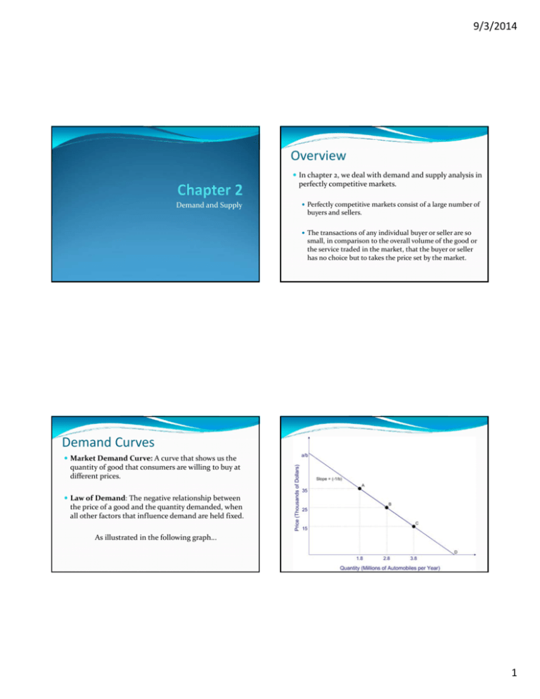
9/3/2014
Overview
 In chapter 2, we deal with demand and supply analysis in perfectly competitive markets. Demand and Supply
 Perfectly competitive markets consist of a large number of buyers and sellers.  The transactions of any individual buyer or seller are so small, in comparison to the overall volume of the good or the service traded in the market, that the buyer or seller has no choice but to takes the price set by the market.
Demand Curves
 Market Demand Curve: A curve that shows us the quantity of good that consumers are willing to buy at different prices.  Law of Demand: The negative relationship between the price of a good and the quantity demanded, when all other factors that influence demand are held fixed.
As illustrated in the following graph… 1
9/3/2014
 The direct demand curve will generally take the linear form…
Example
 Direct Demand Curve: Q = 100 ‐2P
Q -100 = -2p
2P =100 - Q
 Inverse Demand hence becomes:
Q = a – bP
where ‘a’ = vertical intercept, and ‘b’ = slope
 The “Choke Price” is the price at which Q=0, or simply put, at what price consumers demand 0 units of the good. Setting Q=0, the “Choke Price” = 50
Rearranging and solving for P, we get…
Vertical intercept
slope
And so, the graph looks like a straight line . . . a 1
 *Q
b b
This is the Inverse Demand Curve
 Or more generally . . .
Demand: Q = a – bP, then Inverse Demand :
P
Choke Price
(a/b)
P
P
a
b
a Q

b b
0=
a
0
a Q
 Q  a
b a
Q
2
9/3/2014
Supply Curve
 Market Supply Curve: A curve that shows us the total quantity of goods that their suppliers are willing to sell at different prices. Example
Linear Supply Curve: QS = 0.15 + P
 Find the quantity of wheat supplied if… P = $2 → QS = .15 + 2 = 2.15
P = $3 → QS = .15 + 3 = 3.15
 Let us sketch this supply curve…
QS = 0.15 + P and solving for P, we get the inverse supply curve P = QS – 0.15
 So the slope = 1 (coefficient of QS)
 Intercept = ‐0.15
The following figure illustrates this supply curve…
Equilibrium
 In equilibrium, a perfectly competitive market will set a price and quantity such that there is no excess supply and no excess demand, hence demand equals supply. Qs = Qd
 If there is excess supply Qs > Qd → prices should go down
 If there is excess demand Qs< Qd → prices should go up
3
9/3/2014
Example
Inverse Demand Curve →
Demand Curve: Qd = 500 – 4P Supply Curve: QS = ‐100 + 2P
Solving for P:
4p = 500 - Qd
p = 500/4 – Qd /4
Inverse Supply Curve →
Solving for P:
2p = Qs + 100
p = Qs /2 + 50
P = 100
 Before finding the equilibrium output and price level…
Let us sketch these curves on the same graph with quantity on the horizontal axis and price on the vertical axis.
 At what price and quantity do you reach equilibrium?
Q = 100
When P=0, Qd=500‐4.0=500
Comparative Statics: An Increase in Demand, for any given price
QS = Qd
500 – 4P = ‐100 + 2P
600 = 6P
100 = P
 And then take this p=100 and plug it into either the demand or supply curve to find the equilibrium quantity…
P=100
QS = 500 – 4(100) = 100
And so, equilibrium occurs at P=100 and Q=100
4
9/3/2014
A decrease in supply, for any given price
 An increase in demand as the one depicted above can originate from an increase in income, or in the consumer’s preference for the good. For any given price, the quantity that consumers demand has now gone up.  You can visually see that by extending a long horizontal dotted line which maintains your focus on a given (fixed price). The point where the dotted line crosses each demand curve represents the quantity demanded. Example: Market for Aluminum  A decrease in supply might originate from an increase in production costs, which lead producers of the good to supply lower amounts of the good at any given price. [Follow similar graphical representation as above]
Demand: Qd = 500 – 50P + 10I where P=price and I=income
Supply: QS = ‐400 + 50P
 Let’s analyze the equilibrium when income is I=10 and how it is affected when income decreases to I=5
 First, Equilibrium when I = 10…
 Extend a horizontal dotted line at the price p=$10. The quantity supplied is lower after the increase in production costs (S2) than before the increase (S1). Plug in I=10 into Qd to get Qd = 500 – 50P + 10(10) = 600 – 50P
 Equating Qd=QS we obtain…
600‐5p=‐400‐50p
1000=100p
Or p=$10→QS = -400 + 50($10) = 100
5
9/3/2014
 Second, Equilibrium when I = 5…
Qd
Plug I = 5 into Qd to get = 500 – 50P +10(5) = 550 – 50P
 Now equate Qd to QS, Qd
Qs
550 – 50P = ‐400 + 50P
950 + 100P
9.5 = P →QS = ‐400 + 50(9.5) = 75
 (1) Demand shifts inward,  (2) equilibrium output decreases from 100 to 75,  (3) equilibrium price decreases from $10 to $9.50
Query #1
Answer
 Consider the demand Curve
 B, shift to the right
Qd = 1000 ‐20P ‐6r
 If the value of r falls, the demand curve will:
a)Shift to the left b)Shift to the right
c)Remain unchanged
d)Rotate along the quantity axis
 In particular, differentiating the demand function with respect to r,
 ∂Qd/∂r = ‐6<0
 Hence ∆r produces a reduction in Qd and vice versa, a decrease in r produces an increase in Qd
6
9/3/2014
A change in both the demand and supply curve
 A decrease in demand and an increase in supply:
 Unambiguously produce a reduction in the equilibrium price; but…
 the effect on the equilibrium quantity is more ambiguous. In the figure, the outward shift in the supply curve dominates the inward shift in the demand curve, producing an overall increase in the equilibrium quantity. Otherwise, the equilibrium quantity would decrease. Can you draw a figure in which Demand increases and Supply decreases, but equilibrium output decreases? Interpretation…
Price Elasticity of Demand
 We can express the elasticity of demand as…
Now that we know how to construct a demand curve, to what extent does a change in one variable affect quantity demanded?
where
 Price Elasticity of Demand: A measure of the percentage change of quantity demanded as a result of a 1% increase in price, holding all other determinants of demand constant. Q Q1  Q0

Q
Q0
and
P P1  P0

P
P0
Q
P
 Notice that the first term is simply the derivative of quantity demanded with respect to P. Let’s look at an example…
7
9/3/2014
Example
 Suppose that we have a price change that results in the Why is εQ,P always negative?
following changes in quantity demanded…
 When P=10, quantity is Q=50
 When P=12, quantity falls to Q=45 (So ∆Q = ‐5)
 Where
represents the slope of the demand curve, which is negative by the Law of Demand. What is the elasticity of demand?
 Where
∆1% in P ∆0.5% in Q (less-than-proportional decrease)
Example  Let’s look at another example of elasticity…
Demand curve Q = 100 – 2(P)
Hence, the product (‐)٠(+) must be negative, making the elasticity εQ,p a negative number.  Remember that our demand curve is in the form
Q = a – bP, and that the first term of our elasticity equation is simply the derivative with respect to P (i.e., ‐b) so our elasticity equation is…
Q
 2
P
Let’s find the elasticities when . . . Ed 
 A) P=40, so Q= 20
since both p>0 and Q>0.
Q P
*
P Q
 So now, we simply plug in the particular values of P  B) P=25, so Q= 50
and Q to find the elasticity for each price.
 C) P=10, so Q= 80
8
9/3/2014
A) When P=40…
Constant slope (-2), but
not constant elasticity εd
 What about the elasticities for this demand curve at the vertical and horizontal intercepts?  Vertical Intercept
B) When P=25…
 Horizontal Intercept
C) When P=10…
Elasticity of demand in the linear demand curve, Q = a‐bP
P
50
40
25
10
 We can actually summarize where a linear demand will  d  
be…
 d  4
 d  1
 (1) Elastic, when |ε|>1
 (2) Unit Elastic, when |ε|=1
1
d  
4
d  0
 (3) Inelastic, when |ε|<1
Q
9
9/3/2014
Why not use slope of the demand function, rather than EQ, p?
 The reason we use price elasticity of demand (and not simply the slope of the demand curve) is because by using the former we can produce a unit‐free measure of how sensitive is the demand curve to changes in prices. Remember, elasticity of demand does not equal the slope. That is, a linear demand curve (constant slope) can have different elasticities, as we just showed.
 Indeed, note that units cancel out when you use the  In this way we can also compare the sensitivity of formula of price‐elasticity of demand, but they wouldn’t if you were simply using the slope of the demand curve. Qd
Qd in tons
A number
Q
Qin tons
P
P inUS$
P
P inUS$
demand to price changes across different goods:

 Measured in different units (uranium versus steel)
 Consumed in different countries (prices expressed in different currencies)
 Etc…
 We need a unit‐free measure of Qd and Price to be able to compare the changes in one with the changes in the other.
10
9/3/2014
Examples of price‐elasticities of demand:
Cigarettes
‐0.107
Pet food
‐0.061
Air travel, leisure
‐1.52
Air travel, business
‐0.70
Constant Elasticity Demand Curve
 Constant Elasticity Demand Curve:  A demand curve of the form Q = aP‐b where ‘a’ and ‘b’ are positive constants.  The term –b is the price elasticity of demand along all points in this curve.
 Intuition: a 10% increase in the price of cigarettes produces a 1.07% reduction in the quantity demanded. Hence, we can claim that demand for cigarettes is relatively insensitive to price changes. Constant Elasticity Demand Curve
dQ
We will just find dP , and then plug into the  d formula;
 Therefore,
 Let us see why…
 First, recall the formula of price elasticity;
d 
dQ P

dP Q
Query #2
Consider the demand Curve
Qd= 5P‐1
The elasticity of demand along this demand curve:
A. Is inelastic
B. Is elastic
C. Is unitary elastic
D. Falls as the price falls
Q  a * p b
Constant in P
11
9/3/2014
Answer
 C, it is unitary elastic
 The elasticity of demand of a demand curve Qd = A p‐b
is –b
 In this case, Qd =5p‐1, so the exponent ‐1 is the elasticity, which is constant in prices. Different Types of Elasticities of Demand
 So far we have only compared how quantity demanded varies with price, in order to see how price sensitive certain commodities are.  This analysis, however, can be extended to compare more than just quantity with price.
Let’s extend this elasticity analysis to compare Qd with other factors…
What about changes in income? How do they affect demand?
Examples of Income‐elasticity of demand  Apples = 1.32
 Income Elasticity of Demand: The percentage change in quantity demanded resulting from a 1% increase in income, holding price and all other determinants of demand constant.
∆1% in the one produces a 1.32% increase in the
quantity of apples demanded
 Flour = -0.36
∆1% in the one produces a 0.36% decrease in the
quantity of flour demanded
12
9/3/2014
What about changes in the price of other goods? For instance, how the change in the price of Pepsi change the quantity of Coke demanded?
Example of Cross‐Price elasticity of demand (Application 2.4 in textbook)
 ∆1% in the price of Nissan Sentra
 Cross‐Price Elasticity of Demand: The percentage change of the quantity of one good demanded (good i) that results from a 1% increase in the price of another good (good j).
produces a change in the demand of…
Ford Escort
Example of Cross‐Price elasticity of demand (Application 2.4 in textbook)
BMW 735
Application: Coke vs. Pepsi
 ∆1% in the price of Nissan Sentra produces a…
 ∆0.454% in the quantity demanded of Ford Escort
 ∆0% in the quantity demanded of Lexus or BMW 735
 Generally…
 If εQi,Pj >0, goods i and j are regared as substitutes.

(i.e. two brands of mineral water, Nissan Sentra and Ford Escort)
 If εQi,Pj <0, goods i and j are regarded as complements.
 (i.e. left and right shoe, cars and gasoline, etc)
13
9/3/2014
Application: Coke vs. Pepsi
Coke
Pepsi
Price Elasticity of Demand єQ,P
Cross‐Price Elasticity of Demand
Income Elasticity of Demand  Therefore, a ∆1% in the Pcoke produces…

‐1.47
‐1.55
0.52
0.64
1.47% in the quantity demanded of Coke, but…
 ∆0.64% in the quantity demanded of Pepsi
(So people, on average, regard Coke and Pepsi as substitutes!)
 On the other hand, a ∆1% in the income level
produces…
 ∆0.58% in the quantity demanded of coke
0.58
1.38
(You can repeat a similar analysis starting with ∆1% in the
price of Pepsi)
Intuition…
 Back of Envelope calculations about linear  As you might have guessed, we can even extend this analysis to how changes in prices affect the quantity supplied.  This is called the Price Elasticity of Supply.
 It shows us how a 1% change in price affects the amount of the good supplied. Or, how price sensitive is supply?
demand curves:
 Now that we know how a demand curve is constructed and how to use its various parts to analyze the relationship between quantity demanded, quantity supplied, and price, we can work backwards to actually construct a demand curve.
 Consider that we know the prevailing Q, the P, and εQ,P.
We want to find the value of a and b in Q=a-bp, where…
 ‘a’ (vertical intercept or choke price)
 ‘b’ (slope of demand which we can derive from elasticity) Qd =a-bP
14
9/3/2014
We know that, from Q  a  bP,
Q
 b
P
b
 Let’s first find parameter …
Example:  Q=70,
p=$0.70, [Recall that Q= a –bP]
εQ,P =-0.55
 We to find parameters a and b , so we find the demand function
a
-
 Now, let’s find …
 And using the value of b we found above,  (1)
 (2)
 Hence, the demand curve is Qd = 108.5 – 55p
a
b
 Q  (Q,P Q)  a  Q(1  Q,P )
15