Chapter 8
Sampling Distributions
and Estimation
Sampling Variation
• Sample statistic –
Sampling Variation
• a random variable whose value depends
on which population items happen to be
included in the random sample.
sample .
Estimators and Sampling Distributions
Sample Mean and the Central Limit Theorem
Confidence Interval for a Mean (µ
(µ ) with Known σ
Confidence Interval for a Mean (µ
(µ ) with Unknown σ
• Depending on the sample size,
size, the sample
statistic could either represent the population
well or differ greatly from the population.
Confidence Interval for a Proportion (π
(π)
Sample Size Determination for a Mean
Sample Size Determination for a Proportion
C.I. for the Difference of Two Means µ 1 -µ2 (Optional)
C.I. for the Difference of Two Proportions π1 -π2 (Optional)
• This sampling variation can easily be
illustrated.
Confidence Interval for a Population Variance σ2 (Optional)
McGraw- Hill/Irwin
Sampling Variation
Sampling Variation
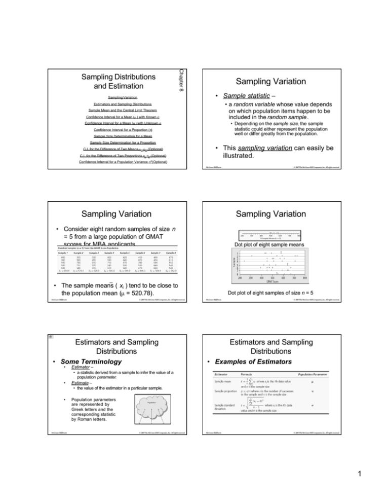
• Consider eight random samples of size n
= 5 from a large population of GMAT
scores for MBA applicants.
Dot plot of eight sample means
• The sample means ( xi ) tend to be close to
the population mean (µ
(µ = 520.78).
McGraw- Hill/Irwin
© 2007 The McGraw-Hill Companies, Inc. All rights reserved.
Dot plot of eight samples of size n = 5
McGraw- Hill/Irwin
Estimators and Sampling
Distributions
• Some Terminology
•
•
•
McGraw- Hill/Irwin
© 2007 The McGraw-Hill Companies, Inc. All rights reserved.
© 2007 The McGraw-Hill Companies, Inc. All rights reserved.
Estimators and Sampling
Distributions
• Examples of Estimators
Estimator –
• a statistic derived from a sample to infer the value of a
population parameter
parameter..
Estimate –
• the value of the estimator in a particular sample.
Population parameters
are represented by
Greek letters and the
corresponding statistic
by Roman letters.
© 2007 The McGraw-Hill Companies, Inc. All rights reserved.
McGraw- Hill/Irwin
© 2007 The McGraw-Hill Companies, Inc. All rights reserved.
1
Estimators and Sampling
Distributions
• Sampling Distributions
•
•
• Bias
The sampling distribution of an estimator is
the probability distribution of all possible
values the statistic may assume when a
random sample of size n is taken.
An estimator is a random variable since
samples vary.
^
• Sampling error = θ – θ
McGraw- Hill/Irwin
Estimators and Sampling
Distributions
• Bias is the difference between the
expected value of the estimator and
the true parameter.
^
• Bias = E( θ ) – θ
• An estimator is unbiased ^if E( θ ) = θ
• On average,
average, an unbiased estimator neither
overstates nor understates the true
parameter.
© 2007 The McGraw-Hill Companies, Inc. All rights reserved.
McGraw- Hill/Irwin
Estimators and Sampling
Distributions
© 2007 The McGraw-Hill Companies, Inc. All rights reserved.
Estimators and Sampling
Distributions
• Bias
• Sampling error is random whereas
bias is systematic
systematic..
• An unbiased estimator avoids systematic
error.
McGraw- Hill/Irwin
© 2007 The McGraw-Hill Companies, Inc. All rights reserved.
McGraw- Hill/Irwin
Estimators and Sampling
Distributions
• Efficiency
•
•
McGraw- Hill/Irwin
© 2007 The McGraw-Hill Companies, Inc. All rights reserved.
Estimators and Sampling
Distributions
• Consistency
Efficiency refers to the variance of the estimator’
estimator’s
sampling distribution.
A more efficient estimator has smaller variance.
© 2007 The McGraw-Hill Companies, Inc. All rights reserved.
• A consistent estimator converges
toward the parameter being estimated
as the sample size increases.
McGraw- Hill/Irwin
© 2007 The McGraw-Hill Companies, Inc. All rights reserved.
2
Sample Mean and the
Central Limit Theorem
• The sample mean is an unbiased
estimator of µ, therefore,
E( X ) = E( X) = µ
Sample Mean and the
Central Limit Theorem
• If the population is exactly normal, then
the sample mean follows a normal
distribution.
• The standard error of the mean is the
standard deviation of the sampling error
σ
of x :
σx =
n
McGraw- Hill/Irwin
© 2007 The McGraw-Hill Companies, Inc. All rights reserved.
McGraw- Hill/Irwin
Sample Mean and the
Central Limit Theorem
•
For example, the average price, µ, of a 5 GB
MP3 player is $80.00 with a standard deviation,
σ, equal to $10.00. What will be the mean and
standard error from a sample of 20 players?
E( X ) = E( X) = µ = $80.00
McGraw- Hill/Irwin
Sample Mean and the
Central Limit Theorem
• Central Limit Theorem (CLT) for a
Mean
•
σ
n
= 10 = $2.236
20
• If the distribution of prices for these players
is a normal distribution, then the sampling
distribution on x is N(80.00, 2.236).
σx =
© 2007 The McGraw-Hill Companies, Inc. All rights reserved.
© 2007 The McGraw-Hill Companies, Inc. All rights reserved.
•
•
McGraw- Hill/Irwin
Sample Mean and the
Central Limit Theorem
If a random sample of size n is drawn from a
population with mean µ and standard
deviation σ, the distribution of the sample
mean x approaches a normal distribution
with mean µ and standard deviation σ x = σ/
n as the sample size increase.
If the population is normal, the distribution of
the sample mean is normal regardless of
sample size.
© 2007 The McGraw-Hill Companies, Inc. All rights reserved.
Sample Mean and the
Central Limit Theorem
• Symmetric Population: Uniform Distribution
•
•
•
McGraw- Hill/Irwin
© 2007 The McGraw-Hill Companies, Inc. All rights reserved.
McGraw- Hill/Irwin
Rule of thumb: to obtain a normal
distribution for the sample mean, n > 30.
A much smaller n will suffice if the population
is symmetric
symmetric..
For example,
consider a
uniform
population
U(500, 1000).
© 2007 The McGraw-Hill Companies, Inc. All rights reserved.
3
Sample Mean and the
Central Limit Theorem
• Symmetric Population: Uniform Distribution
•
The central limit theorem predicts that samples drawn
from this population will have a mean of 1000 and the
standard error of the mean of:
Predicted S.E. for
n=1
σx = σ/ n
= 288.7/ 1 = 288.7
n=2
n=4
= 288.7/ 2 = 204.1
= 288.7/ 4 = 144.3
n = 16
= 288.7/ 16 = 72.2
McGraw- Hill/Irwin
© 2007 The McGraw-Hill Companies, Inc. All rights reserved.
Sample Mean and the
Central Limit Theorem
• Histograms of Sample Means from Uniform
Population
McGraw- Hill/Irwin
Sample Mean and the
Central Limit Theorem
• Histograms of Sample Means from Uniform
Population
McGraw- Hill/Irwin
© 2007 The McGraw-Hill Companies, Inc. All rights reserved.
Sample Mean and the
Central Limit Theorem
• Skewed Population: Waiting Time
• Consider a strongly skewed population
for waiting times
at airport
security
screening
with µ = 2.983
and σ = 2.451
McGraw- Hill/Irwin
Sample Mean and the
Central Limit Theorem
• Skewed Population: Waiting Time
•
The CLT predicts that samples drawn from
this population will have a mean of 2.983
minutes and standard error of the mean:
Predicted S.E. for
n=1
σx = σ/ n
= 2.451/ 1 = 2.451
n=2
n=4
= 2.451/ 2 = 1.733
= 2.451/ 4 = 1.255
n = 16
= 2.451/ 16 = 0.613
McGraw- Hill/Irwin
© 2007 The McGraw-Hill Companies, Inc. All rights reserved.
© 2007 The McGraw-Hill Companies, Inc. All rights reserved.
© 2007 The McGraw-Hill Companies, Inc. All rights reserved.
Sample Mean and the
Central Limit Theorem
• Histograms of Sample Means from Skewed
Population
McGraw- Hill/Irwin
© 2007 The McGraw-Hill Companies, Inc. All rights reserved.
4
Sample Mean and the
Central Limit Theorem
• Histograms of Sample Means from Skewed
Population
Sample Mean and the
Central Limit Theorem
• Range of Sample Means
•
The CLT permits a range or interval within
which the sample means are expected to fall.
Where z is from the
σ
µ+z
standard normal table.
n
• If we know µ and σ, the range of sample means for
samples of size n are predicted to be:
90% Interval
σ
µ + 1.645
n
McGraw- Hill/Irwin
© 2007 The McGraw-Hill Companies, Inc. All rights reserved.
McGraw- Hill/Irwin
Sample Mean and the
Central Limit Theorem
• Illustration: GMAT Scores
•
•
For samples of size n = 5 applicants, within what
range would GMAT means be expected to fall?
The parameters are µ = 520.78 and σ = 86.8. The
predicted range for 95% of the sample means is:
µ + 1.960 σ
n
• The standard error declines as n
increases, but at a decreasing rate.
σ
Make the interval µ + z
n
small by increasing n.
The distribution of
sample means collapses
at the true population
mean µ as n increases.
McGraw- Hill/Irwin
Confidence Interval for a
Mean (µ
(µ) with Known σ
•
•
•
McGraw- Hill/Irwin
© 2007 The McGraw-Hill Companies, Inc. All rights reserved.
Confidence Interval for a
Mean (µ
(µ) with Known σ
• What is a Confidence Interval?
• The confidence interval for µ with known σ is:
• What is a Confidence Interval?
•
© 2007 The McGraw-Hill Companies, Inc. All rights reserved.
• Sample Size and Standard Error
= 520.78 + 1.960 86.8
5
© 2007 The McGraw-Hill Companies, Inc. All rights reserved.
99% Interval
µ + 2.576 σ
n
Sample Mean and the
Central Limit Theorem
= 520.78 + 76.08
McGraw- Hill/Irwin
95% Interval
σ
µ + 1.960
n
A sample mean x is a point estimate of the
population mean µ.
A confidence interval for the mean is a range
µ lower < µ < µ upper
The confidence level is the probability that the confidence
interval contains the true population mean.
The confidence level (usually expressed as a %) is the
area under the curve of the sampling distribution.
© 2007 The McGraw-Hill Companies, Inc. All rights reserved.
McGraw- Hill/Irwin
© 2007 The McGraw-Hill Companies, Inc. All rights reserved.
5
Confidence Interval for a
Mean (µ
(µ) with Known σ
•
• Choosing a Confidence Level
A higher confidence level leads to a wider
confidence interval.
•
Greater confidence implies loss of precision.
•
95% confidence is most often used.
McGraw- Hill/Irwin
© 2007 The McGraw-Hill Companies, Inc. All rights reserved.
Confidence Interval for a
Mean (µ
(µ) with Known σ
• Interpretation
• A confidence interval either does or does
not contain µ.
• The confidence level quantifies the risk .
• Out of 100 confidence intervals,
approximately 95% would contain µ,
while approximately 5% would not
contain µ.
McGraw- Hill/Irwin
Confidence Interval for a
Mean (µ
(µ) with Known σ
• Is σ Ever Known?
Confidence Interval for a
Mean (µ
(µ) with Unknown σ
• Student
Student’’s t Distribution
• Yes, but not very often.
• In quality control applications with
ongoing manufacturing processes,
assume σ stays the same over time.
• In this case, confidence intervals are
used to construct control charts to track
the mean of a process over time.
McGraw- Hill/Irwin
© 2007 The McGraw-Hill Companies, Inc. All rights reserved.
© 2007 The McGraw-Hill Companies, Inc. All rights reserved.
•
x +t
s
n
• The confidence interval for µ (unknown
σ) is x - t s
x +t s
n
<µ<
McGraw- Hill/Irwin
Confidence Interval for a
Mean (µ
(µ) with Unknown σ
• Student
Student’’s t Distribution
Use the Student
Student’’ s t distribution instead of the
normal distribution when the population is
normal but the standard deviation σ is
unknown and the sample size is small.
n
© 2007 The McGraw-Hill Companies, Inc. All rights reserved.
Confidence Interval for a
Mean (µ
(µ) with Unknown σ
• Student
Student’’s t Distribution
• t distributions are symmetric and shaped
like the standard normal distribution.
• The t distribution is dependent on the
size of the sample.
McGraw- Hill/Irwin
© 2007 The McGraw-Hill Companies, Inc. All rights reserved.
McGraw- Hill/Irwin
© 2007 The McGraw-Hill Companies, Inc. All rights reserved.
6
Confidence Interval for a
Mean (µ
(µ) with Unknown σ
• Degrees of Freedom
• Degrees of Freedom
• Degrees of Freedom ( d.f
d.f.)
.) is a parameter
based on the sample size that is used to
determine the value of the t statistic.
• Degrees of freedom tell how many
observations are used to calculate σ, less
the number of intermediate estimates used in
the calculation.
ν=n-1
McGraw- Hill/Irwin
Confidence Interval for a
Mean (µ
(µ) with Unknown σ
© 2007 The McGraw-Hill Companies, Inc. All rights reserved.
• As n increases, the t distribution
approaches the shape of the normal
distribution.
• For a given confidence level, t is always
larger than z , so a confidence interval
based on t is always wider than if z were
used.
McGraw- Hill/Irwin
Confidence Interval for a
Mean (µ
(µ) with Unknown σ
• Comparison of z and t
Confidence Interval for a
Mean (µ
(µ) with Unknown σ
• Comparison of z and t
• For very small samples, t-values differ
substantially from the normal.
• As degrees of freedom increase, the tvalues approach the normal z -values.
• For example, for n = 31, the degrees of
freedom are:
ν = 31 – 1 = 30
• What would the t-value be for a 90%
confidence interval?
McGraw- Hill/Irwin
© 2007 The McGraw-Hill Companies, Inc. All rights reserved.
For ν = 30, the corresponding z -value is 1.645.
McGraw- Hill/Irwin
Confidence Interval for a
Mean (µ
(µ) with Unknown σ
• Example GMAT Scores Again
• Here are the GMAT scores from 20
applicants to an MBA program:
McGraw- Hill/Irwin
© 2007 The McGraw-Hill Companies, Inc. All rights reserved.
© 2007 The McGraw-Hill Companies, Inc. All rights reserved.
© 2007 The McGraw-Hill Companies, Inc. All rights reserved.
Confidence Interval for a
Mean (µ
(µ) with Unknown σ
• Example GMAT Scores Again
• Construct a 90% confidence interval for
the mean GMAT score of all MBA
applicants. x = 510 s = 73.77
• Since σ is unknown, use the Student’
Student ’s t
for the confidence interval with ν = 20 –
1 = 19 d.f
d.f..
• First find t0.90 from Appendix D.
McGraw- Hill/Irwin
© 2007 The McGraw-Hill Companies, Inc. All rights reserved.
7
Confidence Interval for a
Mean (µ
(µ) with Unknown σ
Confidence Interval for a
Mean (µ
(µ) with Unknown σ
• Example GMAT Scores Again
• The 90% confidence interval is:
x-t
513 – 1.729
s
n
<µ<
x +t s
n
73.77
73.77
20 < µ < 513 + 1.729 20
513 – 28.52 < µ < 513 + 28.52
• We are 90% certain that the true mean
GMAT score is within the interval 481.48
< µ < 538.52.
McGraw- Hill/Irwin
Confidence Interval for a
Mean (µ
(µ) with Unknown σ
• Confidence Interval Width
• Confidence interval width reflects
- the sample size,
- the confidence level and
- the standard deviation.
• To obtain a narrower interval and more
precision
- increase the sample size or
- lower the confidence level (e.g., from
90% to
80% confidence)
McGraw- Hill/Irwin
© 2007 The McGraw-Hill Companies, Inc. All rights reserved.
Confidence Interval for a
Mean (µ
(µ) with Unknown σ
• A “Good
Good”” Sample
• Here are five different samples of 25 births
from a population of N = 4,409 births and
their 95% CIs .
McGraw- Hill/Irwin
Confidence Interval for a
Mean (µ
(µ) with Unknown σ
• A “Good
Good”” Sample
© 2007 The McGraw-Hill Companies, Inc. All rights reserved.
Confidence Interval for a
Mean (µ
(µ) with Unknown σ
• Using Appendix D
• An examination of the samples shows
that sample 5 has an outlier.
• The outlier is a warning that the resulting
confidence interval possibly could not be
trusted.
• In this case, a larger sample size is
needed.
McGraw- Hill/Irwin
© 2007 The McGraw-Hill Companies, Inc. All rights reserved.
© 2007 The McGraw-Hill Companies, Inc. All rights reserved.
• Beyond ν = 50, Appendix D shows ν in
steps of 5 or 10.
• If the table does not give the exact
degrees of freedom, use the t-value for
the next lower ν.
• This is a conservative procedure since it
causes the interval to be slightly wider.
• For d.f
d.f.. above 150, use the z -value.
McGraw- Hill/Irwin
© 2007 The McGraw-Hill Companies, Inc. All rights reserved.
8
Confidence Interval for a
Mean (µ
(µ) with Unknown σ
• Using Excel
Confidence Interval for a
Mean (µ
(µ) with Unknown σ
• Using MegaStat
• Use Excel’
Excel’s function =TINV(probability
=TINV(probability , d.f
d.f.)
.) to obtain
a twotwo-tailed value of t. Here, “probability ” is 1 minus
the confidence level.
McGraw- Hill/Irwin
© 2007 The McGraw-Hill Companies, Inc. All rights reserved.
• MegaStat give you a choice of z or t and
does all calculations for you.
McGraw- Hill/Irwin
Confidence Interval for a Proportion
(π )
•
A proportion is a mean of data whose only
value is 0 or 1.
•
The Central Limit Theorem (CLT) states that
the distribution of a sample proportion p = x /n
approaches a normal distribution with mean π
and standard deviation
σp =
•
McGraw- Hill/Irwin
Confidence Interval for a Proportion
(π )
• Illustration: Internet Hotel Reservations
•
•
p = x /n is a consistent estimator of π.
McGraw- Hill/Irwin
Confidence Interval for a Proportion
(π )
• Illustration: Internet Hotel Reservations
• Here are five random samples of n = 20.
Each p is a point estimate of π.
• Notice the sampling variation in the
value of p.
McGraw- Hill/Irwin
Management of the PanPan- Asian Hotel System
tracks the percent of hotel reservations made
over the Internet.
The binary data are:
1 Reservation is made over the Internet
0 Reservation is not made over the Internet
After data was collected, it was determined that
the proportion of Internet reservations is π =
.20.
•
π(1
(1--π)
n
© 2007 The McGraw-Hill Companies, Inc. All rights reserved.
© 2007 The McGraw-Hill Companies, Inc. All rights reserved.
Confidence Interval for a Proportion
(π )
• Applying the CLT
•
The distribution of
a sample
proportion p = x /n
is symmetric if π
= .50 and
regardless of π,
approaches
symmetry as n
increases.
McGraw- Hill/Irwin
© 2007 The McGraw-Hill Companies, Inc. All rights reserved.
9
Confidence Interval for a Proportion
(π )
• Applying the CLT
•
• When is it Safe to Assume Normality?
As n increases, the statistic p = x /n more
closely resembles a continuous random
variable.
As n increases, the distribution becomes more
symmetric and bell shaped.
As n increases, the range of the sample
proportion p = x /n narrows.
The sampling variation can be reduced by
increasing the sample size n.
•
•
•
McGraw- Hill/Irwin
© 2007 The McGraw-Hill Companies, Inc. All rights reserved.
Confidence Interval for a Proportion
(π )
• Standard Error of the Proportion
•
The standard error of
the proportion σ p
depends on π, as
well as n.
•
It is largest when π is
near .50 and smaller
when π is near 0 or
1.
McGraw- Hill/Irwin
Confidence Interval for a Proportion
(π )
•
Rule of Thumb: The sample proportion p = x /n
may be assumed to be normal if both nπ > 10
and
n(1
(1-- π) > 10.
Sample size to
assume normality:
McGraw- Hill/Irwin
Confidence Interval for a Proportion
(π )
• Standard Error of the Proportion
•
© 2007 The McGraw-Hill Companies, Inc. All rights reserved.
Confidence Interval for a Proportion
(π )
• Standard Error of the Proportion
• Enlarging n reduces the standard
error σp but at a diminishing rate.
© 2007 The McGraw-Hill Companies, Inc. All rights reserved.
The formula for the standard error is
symmetric.
McGraw- Hill/Irwin
© 2007 The McGraw-Hill Companies, Inc. All rights reserved.
Confidence Interval for a Proportion
(π )
• Confidence Interval for π
• The confidence interval for π is
π+z
π(1
(1--π)
n
Where z is based on the desired confidence.
• Since π is unknown, the confidence interval for
p = x / n (assuming a large sample) is
p+z
McGraw- Hill/Irwin
© 2007 The McGraw-Hill Companies, Inc. All rights reserved.
McGraw- Hill/Irwin
p(1
(1-- p)
n
© 2007 The McGraw-Hill Companies, Inc. All rights reserved.
10
Confidence Interval for a Proportion
(π )
• Confidence Interval for π
Confidence Interval for a Proportion
(π )
• Example Auditing
• z can be chosen for any confidence
level.
For example,
•
A sample of 75 retail inin-store purchases showed that
24 were paid in cash. What is p?
p = x /n = 24/75 = .32
• Is p normally distributed?
np = (75)(.32) = 24
n(1
(1-- p) = (75)(.88) = 51
Both are > 10, so we may conclude normality.
McGraw- Hill/Irwin
© 2007 The McGraw-Hill Companies, Inc. All rights reserved.
Confidence Interval for a Proportion
(π )
• Example Auditing
•
p(1
(1-- p)
n
.32(1-.32)
.32(175
= .32 + 1.96
= .32 + .106
.214 < π < .426
• We are 95% confident that this interval
contains the true population proportion.
McGraw- Hill/Irwin
© 2007 The McGraw-Hill Companies, Inc. All rights reserved.
Confidence Interval for a Proportion
(π )
• Narrowing the Interval
The 95% confidence interval for the proportion of
retail inin-store purchases that are paid in cash is:
p+z
McGraw- Hill/Irwin
© 2007 The McGraw-Hill Companies, Inc. All rights reserved.
Confidence Interval for a Proportion
(π )
• Using Excel and MegaStat
• To find a confidence interval for a
proportion in Excel, use (for example)
• The width of the confidence interval
for π depends on
- the sample size
- the confidence level
- the sample proportion p
• To obtain a narrower interval (i.e.,
more precision) either
- increase the sample size
- reduce the confidence level
McGraw- Hill/Irwin
© 2007 The McGraw-Hill Companies, Inc. All rights reserved.
Confidence Interval for a Proportion
(π )
• Using Excel and MegaStat
• In MegaStat, enter p and n to obtain
the confidence interval for a
proportion.
=0.15-NORMSINV(.95)*SQRT(0.15*(1
=0.15NORMSINV(.95)*SQRT(0.15*(1-0.15)/200)
=0.15+NORMSINV(.95)*SQRT(0.15*(1=0.15+NORMSINV(.95)*SQRT(0.15*(10.15)/200)
McGraw- Hill/Irwin
© 2007 The McGraw-Hill Companies, Inc. All rights reserved.
• MegaStat always assumes normality.
McGraw- Hill/Irwin
© 2007 The McGraw-Hill Companies, Inc. All rights reserved.
11
Confidence Interval for a Proportion
(π )
• Using Excel and MegaStat
•
Confidence Interval for a Proportion
(π )
• Polls and Margin of Error
•
If the sample is small, the distribution of p
may not be well approximated by the normal.
Confidence limits around p can be
constructed by using the binomial distribution.
•
McGraw- Hill/Irwin
© 2007 The McGraw-Hill Companies, Inc. All rights reserved.
•
• Each reduction in the margin of error
requires a disproportionately larger
sample size.
McGraw- Hill/Irwin
Sample Size Determination for a
Mean
• Sample Size to Estimate µ
•
© 2007 The McGraw-Hill Companies, Inc. All rights reserved.
Sample Size Determination for a
Mean
• How to Estimate σ ?
To estimate a population mean with a
precision of + E (allowable error), you would
need a sample of size
n = zσ
E
In polls and surveys, the confidence interval width
when π = .5 is called the margin of error.
error.
Below are some margins of error for 95% confidence
interval assuming π = .50.
• Method 1: Take a Preliminary Sample
Take a small preliminary sample and use
the sample s in place of σ in the sample
size formula.
2
• Method 2: Assume Uniform Population
Estimate rough upper and lower limits a
and b and set σ = [(b
[(b -a)/12]½ .
McGraw- Hill/Irwin
© 2007 The McGraw-Hill Companies, Inc. All rights reserved.
McGraw- Hill/Irwin
Sample Size Determination for a
Mean
• How to Estimate σ ?
•
Sample Size Determination for a
Mean
• Using MegaStat
Method 3: Assume Normal Population
Estimate rough upper and lower limits a and b and
set σ = (b
(b-a)/4. This assumes normality with most of
the data with µ + 2σ so the range is 4σ
4σ.
• Method 4: Poisson Arrivals
In the special case when µ is a Poisson arrival
rate, then σ = µ
McGraw- Hill/Irwin
© 2007 The McGraw-Hill Companies, Inc. All rights reserved.
© 2007 The McGraw-Hill Companies, Inc. All rights reserved.
•
There is a
sample size
calculator in
MegaStat.
The Preview
button lets
you change
the setup and
see results
immediately.
McGraw- Hill/Irwin
© 2007 The McGraw-Hill Companies, Inc. All rights reserved.
12
Sample Size Determination for a
Mean
Sample Size Determination
for a Proportion
• To estimate a population proportion with
a precision of + E (allowable error), you
would need a sample of size
• Caution 1: Units of Measure
•
When estimating a mean, the allowable error E
is expressed in the same units as X and σ.
• Caution 2: Using z
n=
• Using z in the sample size formula for a
mean is not conservative.
• Caution 3: Larger n is Better
• The sample size formulas for a mean tend
to underestimate the required sample
size. These formulas are only minimum
guidelines.
McGraw- Hill/Irwin
© 2007 The McGraw-Hill Companies, Inc. All rights reserved.
•
Method 1: Take a Preliminary Sample
Take a small preliminary sample and use the sample p
in place of π in the sample size formula.
Method 2: Use a Prior Sample or Historical Data
How often are such samples available? π might be
different enough to make it a questionable assumption.
Method 3: Assume that π = .50
This conservative method ensures the desired precision.
However, the sample may end up being larger than
necessary.
•
•
McGraw- Hill/Irwin
π(1
(1-- π)
McGraw- Hill/Irwin
© 2007 The McGraw-Hill Companies, Inc. All rights reserved.
Sample Size Determination
for a Proportion
• Caution 1: Units of Measure
•
For a proportion, E is always between 0 and 1.
For example,
example, a 2% error is E = 0.02.
• Caution 2: Finite Population
• For a finite population, to ensure that the
sample size never exceeds the population
size, use the following adjustment:
n' =
nN
n + (N
(N- 1)
© 2007 The McGraw-Hill Companies, Inc. All rights reserved.
Confidence Interval for the Difference
of Two Means, µ1 – µ 2
• If the confidence interval for the difference of
two means includes zero, we could conclude
that there is no significant difference in means.
• The procedure for constructing a confidence
interval for µ1 – µ 2 depends on our assumption
about the unknown variances.
• Assuming equal variances:
(x 1 – x 2) + t
( n1 – 1)
1)ss 12 + (n
(n2 – 2)
2)ss 22
n1 + n2 - 2
1 +1
n1 n2
with ν = (n
(n1 – 1) + (n
(n2 – 1) degrees of freedom
McGraw- Hill/Irwin
2
• Since π is a number between 0 and 1,
the allowable error E is also between 0
and 1.
Sample Size Determination
for a Proportion
• How to Estimate π?
z
E
© 2007 The McGraw-Hill Companies, Inc. All rights reserved.
Confidence Interval for the Difference
of Two Means, µ1 – µ2
• Assuming unequal variances:
(x 1 – x 2) + t
with ν' =
s 12 s 22
+
n1 n2
[s 12/n1 + s 22/n2]2
(Welch’’s formula for
(Welch
( s 12/n1) 2 + (s
(s 22/n2) 2 degrees of freedom)
n1 – 1
n2 – 1
Or you can use a conservative quick rule for the
degrees of freedom: ν* = min (n
(n1 – 1, n2 – 1).
McGraw- Hill/Irwin
© 2007 The McGraw-Hill Companies, Inc. All rights reserved.
13
Confidence Interval for the Difference
of Two Proportions, π 1 – π2
• If both samples are large (i.e., np > 5 and
n(1
(1--p) > 5, then a confidence interval for
the difference of two sample proportions
is given by
( p1 – p2) + z
McGraw- Hill/Irwin
p1(1 - p1) + p2(1 - p2)
n1
n2
© 2007 The McGraw-Hill Companies, Inc. All rights reserved.
14