MatLab Programming – Lesson 4: Mini-projects
1) Log into your computer and open MatLab…
2) If you don’t have the previous M-scripts saved, you can find them at
http://www.physics.arizona.edu/~physreu/dox/matlab_lesson_1.pdf,
http://www.physics.arizona.edu/~physreu/dox/matlab_lesson_2.pdf, and
http://www.physics.arizona.edu/~physreu/dox/matlab_lesson_3.pdf.
You have now been exposed to all the major programming aspects of MatLab. What remains is
having practice using these tools. It is important that you be able to 1) program logic, 2) handle data and
3) visualize results.
Programming logic accurately is crucial to getting to the truth as well as maximizing your
computational resources. Handling data is important (and often frustrating) so that you can use your
program’s results. Finally, being able to make attractive looking graphics whether in published papers,
grant proposals, scholarship applications, or homework is your chance to set yourself apart from the rest
of your competitors. So many times others will be much more attentive to your work when you can show
your science/technology rather than just telling them.
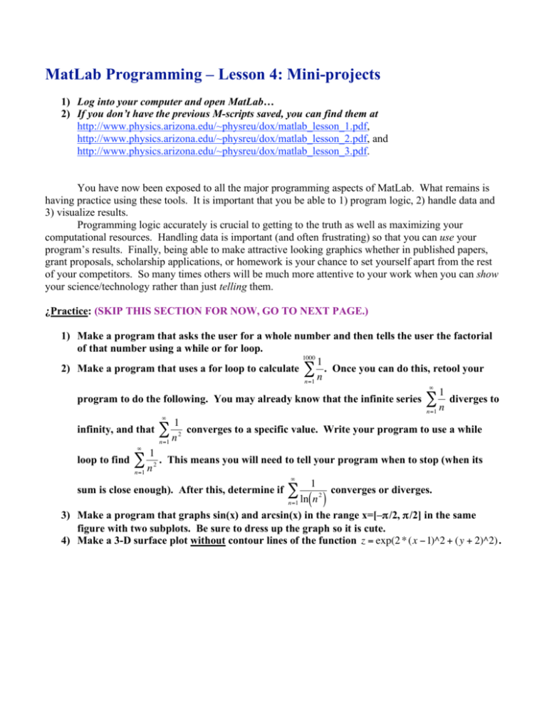
¿Practice: (SKIP THIS SECTION FOR NOW, GO TO NEXT PAGE.)
1) Make a program that asks the user for a whole number and then tells the user the factorial
of that number using a while or for loop.
1000
1
2) Make a program that uses a for loop to calculate " . Once you can do this, retool your
n=1 n
"
1
program to do the following. You may already know that the infinite series # diverges to
n=1 n
"
1
!
infinity, and that # 2 converges to a specific
value. Write your program to use a while
n=1 n
"
1
!
loop to find # 2 . This means you will need to tell your program when to stop (when its
n
n=1
"
1
!
sum is close enough). After this, determine if #
converges or diverges.
2
n=1 ln( n )
3) Make
! a program that graphs sin(x) and arcsin(x) in the range x=[–π/2, π/2] in the same
figure with two subplots. Be sure to dress up the graph so it is cute.
4) Make a 3-D surface plot without contour lines of the function z = exp(2 * (x "1)^2 + (y + 2)^2) .
!
!
Editing Others’ Programs
Finally, when you enter a new lab, you usually inherit programming code that you must figure
out and then modify. On the next several pages is a MatLab program wherein zombies attack
people who are close to them, but rot to uselessness after 100 minutes. Answer the questions
about the program that follow it. (You also may find it easiest to print the program out for ease
of viewing when answering the questions that follow.)
%% Zombie attack model can also be retooled for gaseous
%% diffusion or chemical reactions.
close all; clear all; clc; format long e;
set(gcf,'units','normalized','position',[.1,.1,.8,.8]);
set(0,'defaultaxesfontsize',15);
set(0,'defaulttextfontsize',15);
set(0,'defaultlinelinewidth',3);
% Another slick way to control graphics (play with it).
fprintf('The room is 10x10 and there is a zombie in it!\n\n');
time = 0;
%% Set up arrays for zombies' and people's coordinates (2-D).
number_of_people = ...
input('How many people are in the room (at least 1, try 200).\n');
zombies = [10*rand(1,2),time];
rotten_zombies = [];
number_of_zombies = 1;
people = zeros(number_of_people,2);
for i_people = 1:number_of_people,
people(i_people,:) = 10*rand(1,2);
end;
%% Make initial graph.
plot(people(:,1),people(:,2),'yp',...
'markerfacecolor','y','markersize',12,'linewidth',1);
title(['Time = ',num2str(time),' minutes']);
hold on;
plot(zombies(:,1),zombies(:,2),'rs',...
'markerfacecolor','r','markersize',14,'linewidth',1);
whitebg([0,0,0]);
drawnow;
hold off;
clc;
fprintf('Press a key to let the infection begin!\n\n');
pause();
clc;
%% Begin zombie machine.
stop = ['n'];
safety_exit = 0;
infected = [];
while stop == 'n';
if safety_exit > 5,
break;
end;
safety_exit = safety_exit + 1;
time = time + 1;
for i_auto=1:10000,
%% Make them walk a little.
people = people + 0.1*rand(number_of_people,2)-.05;
zombies = zombies + ...
[[0.2*rand(number_of_zombies,2)-.1],[ones(number_of_zombies,1)]];
%% Make them stay in [0,10]x[0,10] by bouncing off walls.
for i_people = 1:number_of_people,
if people(i_people,1) < 0,
people(i_people,1) = -1*people(i_people,1);
elseif people(i_people,1) > 10,
people(i_people,1) = 20 - people(i_people,1);
end;
if people(i_people,2) < 0,
people(i_people,2) = -1*people(i_people,2);
elseif people(i_people,2) > 10,
people(i_people,2) = 20 - people(i_people,2);
end;
end;
for i_zombie = 1:number_of_zombies,
if zombies(i_zombie,1) < 0,
zombies(i_zombie,1) = -1*zombies(i_zombie,1);
elseif zombies(i_zombie,1) > 10,
zombies(i_zombie,1) = 20 - zombies(i_zombie,1);
end;
if zombies(i_zombie,2) < 0,
zombies(i_zombie,2) = -1*zombies(i_zombie,2);
elseif zombies(i_zombie,2) > 10,
zombies(i_zombie,2) = 20 - zombies(i_zombie,2);
end;
end;
%% Find who is too close to zombie.
for i_people = 1:number_of_people,
for i_zombie = 1:number_of_zombies,
if sqrt((people(i_people,1)-zombies(i_zombie,1)).^2 + ...
(people(i_people,2)-zombies(i_zombie,2)).^2) < .6,
infected(end+1) = i_people;
break;
end;
end;
end;
%% Change infected people from 'people' to 'zombies'.
if size(infected,2) > 0,
infected = fliplr(infected);
for i_infected=1:size(infected,2),
zombies(end+1,:) = ...
[[people(infected(i_infected),:)],[0]];
people(infected(i_infected),:) = [];
end;
number_of_zombies = size(zombies,1);
number_of_people = size(people,1);
infected = [];
end;
%% Change 'zombies' to 'rotten_zombies' if they are around
%% too long.
for i_rotten=number_of_zombies:-1:1,
if zombies(i_rotten,3) > 99;
rotten_zombies(end+1,:) = zombies(i_rotten,1:2);
zombies(i_rotten,:) = [];
end;
end;
number_of_zombies = size(zombies,1);
%% Quit if no people left.
if size(people,1) == 0,
disp(['Complete bloodbath in ',num2str(time),' minutes.']);
return;
end;
%% Quit if no zombies left.
if size(zombies,1) == 0,
disp(['People survive after ',num2str(time),' minutes!']);
return;
end;
%% Update graph of room.
time = time + 1;
plot(people(:,1),people(:,2),'yp',...
'markerfacecolor','y','markersize',12,'linewidth',1);
title(['Time = ',num2str(time),' minutes']);
hold on;
plot(zombies(:,1),zombies(:,2),'rs',...
'markerfacecolor','r','markersize',14,'linewidth',1);
if size(rotten_zombies,1) > 0,
plot(rotten_zombies(:,1),rotten_zombies(:,2),'gs',...
'markerfacecolor','g','markersize',14,'linewidth',1);
end;
whitebg([0,0,0]);
drawnow;
hold off;
pause(.001);
end;
clc;
stop = input('Stop attack? (Y/n).\n','s');
end;
Zombie Questions
Can you understand someone else’s code? Often in research you must learn how to use a previous
student’s program. Test your skills at modifying other’s programs. Change the previous zombie
program to answer the following:
1) Figure out how to make the zombies walk twice as fast as they do currently.
2) Figure out how to let the zombies turn people into other zombies if they are at a distance of 0.75.
3) Figure out how to make the zombies live for 200 minutes.
4) With these new settings, what seems to be the right number of people in the room so that people
survive half of the time that the program is run?
________________________ people.
5) Figure out how to make a gray background for the graph. (Hint: you may need to read
“colors::typical RGB values” in the help menu.)
6) Bonus: make a program to model a haunted house with werewolves and vampires!
Check your solutions with your neighbors, but do not eat their brains!
Projectile Motion
In order to model projectile motion, you need to find the forces on the projectile and use them to calculate
the projectiles:
1) x-position,
2) y-position,
3) x-velocity,
4) y-velocity,
5) x-acceleration, and
6) y-acceleration.
To do this you need to know:
1) the initial x-position,
2) the initial y-position,
3) the initial x-velocity,
4) the initial y-velocity,
5) the time interval between calculation steps,
6) the mass of the projectile,
7) the high-velocity air drag (we can ignore air viscosity since its not sticky like honey)
a) the projectile’s cross sectional area, A,
b) the density of air, ρ,
c) the projectile’s drag/aerodynamic coefficient, Cdrag, (assume 0.5 for a smooth ball, but
0.3 for a baseball or any ball with a surface that breaks up the wake behind the ball).
r
1
d) high velocity drag equation: Fhigh v = "Cdrag #Av 2 vˆ (opposite direction of velocity) ,
2
drag
8) gravitational acceleration, and
9) loops to step by step compute the trajectory in both the x and y direction.
!
Here is a bare bones version for you to begin playing with:
%% Name of team, date, etc. Always give program author.
%% Purpose of program.
%% Be sure to comment well.
close all; clear all; clc; format long e;
%%
%%
%%
%%
Work in SI units.
My catapult launches from a height of 3/4 meters (see y_0 below).
Remember that 10 m/s is about 20 miles per hour.
One tenth second time steps is most likely too large.
x_0 = 0; % 1) the initial x-position,
y_0 = .75; % 2) the initial y-position,
v_x_0 = 20; % 3) the initial x-velocity, you have to estimate
v_y_0 = 10; % 4) the initial y-velocity, you have to estimate
dt = 0.1; % 5) the time interval between calculation steps
mass = 0.042; % 6) the mass of the projectile. Found online for
racquetball.
Area = 1.02e-2; % a) the projectile’s cross sectional area, A,
rho = 1.2; % b) the density of air
C_drag = 0.5; % c) the projectile’s drag/aerodynamic coefficient, Cdrag,
g = 9.8; % 8) gravity,
%% How many iterations will you run?
N_steps = 100; % Make large enough for projectile to strike ground.
%% Now define arrays that will hold data.
x = zeros(1,N_steps + 1); % 1) x-position,
x(1) = x_0; % Make sure initial value is correct.
y = zeros(1,N_steps + 1); % 2) y-position,
y(1) = y_0; % Make sure initial value is correct.
v_x = zeros(1,N_steps + 1); % 3) x-velocity,
v_x(1) = v_x_0; % Make sure initial value is correct.
v_y = zeros(1,N_steps + 1); % 4) y-velocity,
v_y(1) = v_y_0; % Make sure initial value is correct.
%% Use formulas for acceleration later, just define as 0 for now.
a_x = 0; % 5) x-acceleration,
a_y = 0; % 6) y-acceleration.
angle = tan(v_y_0 / v_x_0); % Defining the trajectory angle will save on
thinking.
%{
Note that a_drag has x and y components, and that a_drag is given by
a_drag_x = -C_drag*.5*rho*Area*(v_x^2 + v_y^2)/mass*cos(angle) and
a_drag_y = -C_drag*.5*rho*Area*(v_x^2 + v_y^2)/mass*sin(angle).
%}
%% Now make loop to calculate the data based upon the forces.
i_loop = 1;
n_loop = 1;
while i_loop < N_steps, % Skip the initial values.
angle = tan(v_y(i_loop) / v_x(i_loop))
a_x = -C_drag*.5*rho*Area*(v_x(i_loop)^2 +
v_y(i_loop)^2)/mass*cos(angle);
v_x(i_loop+1) = v_x(i_loop) + a_x*dt; % Remember: v = v_o + a*t
x(i_loop + 1) = x(i_loop) + v_x(i_loop)*dt + .5*a_x*dt^2; % Rem:
x=x_o+v_o*t+.5a*t^2
a_y = -g - C_drag*.5*rho*Area*(v_x(i_loop)^2 +
v_y(i_loop)^2)/mass*sin(angle);
v_y(i_loop +1) = v_y(i_loop) + a_y*dt; % Remember: v = v_o + a*t
y(i_loop + 1) = y(i_loop) + v_y(i_loop)*dt + .5*a_y*dt^2; % Rem:
y=y_o+v_o*t+.5a*t^2
%% If the projectile passes below the ground, we want to stop.
if y(i_loop+1) < 0,
i_loop = N_steps;
n_loop = n_loop+1;
else,
i_loop = i_loop+1;
n_loop = n_loop+1;
end;
end;
%{
If we leave the loop early because the ball is lower than the ground,
we want to delete the extra data that is still stored as zeros.
%}
if n_loop < N_steps,
x(n_loop:end) = [ ]; % Empties out rest of array.
y(n_loop:end) = [ ];
end;
%% Now make graph.
plot(x,y,'r-'); % Make an attractive graph and save as a jpg.
(END OF LESSON 4)