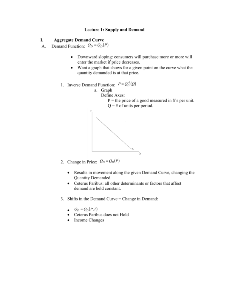
Lecture 1: Supply and Demand
I.
A.
Aggregate Demand Curve
Demand Function: QD  QD P 


Downward sloping: consumers will purchase more or more will
enter the market if price decreases.
Want a graph that shows for a given point on the curve what the
quantity demanded is at that price.
1. Inverse Demand Function: P  QD Q
a. Graph
Define Axes:
P = the price of a good measured in $’s per unit.
Q = # of units per period.
1
2. Change in Price: QD  QD P 


Results in movement along the given Demand Curve, changing the
Quantity Demanded.
Ceterus Paribus: all other determinants or factors that affect
demand are held constant.
3. Shifts in the Demand Curve = Change in Demand:



QD  QD P, I 
Ceterus Paribus does not Hold
Income Changes

Prices of Related Goods
 Let there be two goods: X & Y.
 Complements – similar movement:
Py  Qy  & Qx 
 Substitutes – opposite movement
Py  Qy  & Qx 
II.
Aggregate Supply Curve
A. Supply Function: QS  QS P 

Upward Sloping: The higher the price the more firms are
willing to produce because they can cover the higher opportunity costs
(such as the increased use of labor and capital) to increase production.

A given point on the curve tells us what the quantity supplied is
at that price.
Demand Schedule:
P
.75
.80
.85
.90
Mathematically:
Direct:
Inverse:
1.
Qd
225
250
275
300
Qs
150
200
250
300
Qd = 750 – 500 P
Qs = -600 + 1000 P
P = 3/2 – 1/500 Qd
P = -3/5 + 1/1000 Qs
1
Inverse Supply Function: P  QS Q
a. Graph
2. Change in Price: QS  QS P 


Gives movement along the given Supply Curve, changing the
Quantity Supplied.
Ceterus Paribus: all other determinants or factors that affect supply
are held constant.
3. Shifts in the Supply Curve = Change in Supply: QS  QS P, w, r 




Ceterus Paribus does not Hold
See a change in the quantity supplied across all market prices.
Technology Changes
Input Supply
Other Factors: Population, Preferences, Expectations,
III.
Determination of Equilibrium Price and Quantity
A. Graph: Equilibrium.

Market Clearing: Point at which the quantity supplied equals the
quantity demanded
B.
Example: Equilibrium in the Wheat market
A statistical study of wheat prices and quantities from 1981 showed the
supply and demand curves to be:
QS = 1800 + 240P
QD = 3550 - 266P
IV.
Adjustment to Changes in Demand or Supply

Ceterus Paribus does not hold, curves shift
A.
Market Mechanism
i) Leads to a new equilibrium price and quantity.
ii) Tendency of market towards a clearing price.

Assumes Competitive Markets: Sellers and Buyers do not have
market power.


Disequilibria puts pressure on prices to adjust
 Shortage: QD  QS at price P0.
 Surplus: QD  QS at price P0.
Example: Market Adjustment After a Shift in Demand
o
The price of corn decreases – the demand curve for
wheat shifts back




At 1, we are at the original equilibrium.
At 2, for price P* surplus results at the original price.
At 3, price must decrease to P*’.
Wheat Example Continued
New Demand: QD = 2580 - 194P
New market clearing price:
1800 + 240P = 2580 – 194P
P=
B.
Market Intervention: can prevent prices from adjusting

Price Ceiling

C.
V.
Price Floor
o
Farmer price supports
o
An example of a wheat price floor
Market Mechanism with a Shift in Both Supply and Demand

The ambiguity of price/quantity directions.

Let D & S shift out

Think about how this price ambiguity relates to.
Price Elasticity of Demand

Elasticity measures the sensitivity of one variable to another.
A. Price Elasticity of Demand: The percentage change in quantity demanded
divided by the percentage change in price

Measures the responsiveness of quantity demanded to a change in
the product’s price.
o
Along the Demand curve.
o
The percent change in quantity from a 1 % increase in price.

The relationship is always negative.
o
Convention just leaves off the sign.

The Types of Price Elasticity
 Elastic: E p  1


Inelastic: E p  1

Unit Elastic: E p  1
Price Elasticity Formula:
 Q 
Q  Q P
%Q 
Ep 




P
%P
P Q
P


o
Elasticity can change when moving along the demand curve:
Therefore the point elasticity formula is for a small change in price and
quantity.
B.
C.
Application: How price elasticity affects the total revenue to the firm.
a.
Total Revenue: TR = P x Q
b.
In an Elastic market:
% decrease in Q > % increase in P → decrease in TR
c.
In an Inelastic market:
% decrease in Q < % increase in P → increase in TR
Long run and Short run Demand.

Generally, demand is more price elastic in the long run than in
the short run.
 In long run, consumers can find more substitutes or change
their consumption.

Exception: Durable goods
 People must purchase the item in the long run.
 Durable goods have a more price elastic demand in the short
run.
D.
Problem
The table shows the retail price and sales for instant coffee and roasted coffee for
1997 and 1998.
Year
1997
Retail Price of Sales of Instant
Instant Coffee
Coffee
($/lb)
(million lbs)
10.35
75
Retail Price of
Roasted Coffee
($/lb)
4.11
Sales of Roasted
Coffee
(Million lbs)
820
1998
10.48
3.76
850
70
a.
Using this data alone, estimate the short run price elasticity of
demand for roasted coffee. Also, derive a linear demand curve for
roasted coffee.
To find elasticity, first estimate the slope of the demand curve:
Q
P

Given the slope, we can now estimate elasticity using the price and
quantity data from the table. Since the demand curve is assumed
to be linear, the elasticity will differ in 1997 and 1998 because
price and quantity are difference. You can calculate the elasticity
at both points and at the average point between the two years:
E 97
p 
P Q
Q P

E 98
p 
P Q
Q P

E
AVE
p

P97  P98
2
Q97  Q98
2
Q

P
To derive the demand curve for roasted coffee, note that the slope
of the demand curve and the coefficient a, use the data points from
the table above.
The equation for the demand curve is therefore: