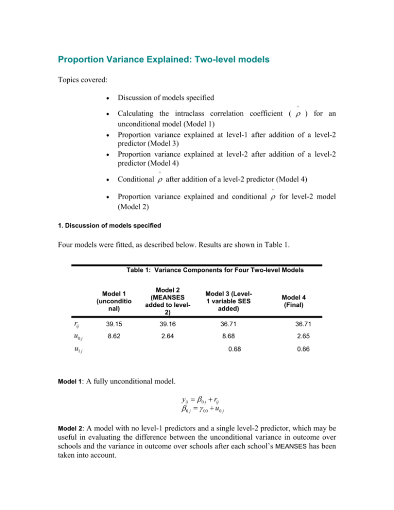
Proportion Variance Explained: Two-level models
Topics covered:

Discussion of models specified

Calculating the intraclass correlation coefficient (  ) for an
unconditional model (Model 1)
Proportion variance explained at level-1 after addition of a level-2
predictor (Model 3)
Proportion variance explained at level-2 after addition of a level-2
predictor (Model 4)


^
^

Conditional  after addition of a level-2 predictor (Model 4)

Proportion variance explained and conditional  for level-2 model
(Model 2)
^
1. Discussion of models specified
Four models were fitted, as described below. Results are shown in Table 1.
Table 1: Variance Components for Four Two-level Models
Model 1
(unconditio
nal)
Model 2
(MEANSES
added to level2)
Model 3 (Level1 variable SES
added)
rij
39.15
39.16
36.71
36.71
u0 j
8.62
2.64
8.68
2.65
u1 j
0.68
Model 4
(Final)
0.66
Model 1: A fully unconditional model.
yij   0 j  rij
 0 j   00  u0 j
Model 2: A model with no level-1 predictors and a single level-2 predictor, which may be
useful in evaluating the difference between the unconditional variance in outcome over
schools and the variance in outcome over schools after each school’s MEANSES has been
taken into account.
yij   0 j  rij
 0 j   00   01 ( MEANSES ) j  u0 j
Model 3: Random-intercept-and-slope model with a group-mean centered level-1
predictor.
yij   0 j  1 j ( SES )ij  rij
 0 j   00  u0 j
1 j   10  u1 j
Model 4: The final model, containing both level-1 predictor and conditional random slope
and intercept coefficient at level-2.
yij   0 j  1 j ( SES )ij  rij
 0 j   00   01 ( MEANSES ) j  u0 j
1 j   10   11 ( MEANSES ) j  u1 j
^
2. Calculating the intraclass correlation coefficient (  ) for an unconditional model (Model
1)
In the unconditional model, the total variation in outcome can be clearly divided between
variation over students and variance on a school level.  2 represents the total variance in
outcomes within school that can be explained by a level-1 model, while  00 is the total
explainable variation at level-2 (schools). As such, this model serves as baseline for
comparison with subsequent, more complex models.
The intraclass correlation coefficient represents the proportion of the variance in outcome
between the schools:
^
 00
^

^
^ 2
 00  

8.62
 0.1804
8.62  39.15
18% of the variance is thus over schools, and the remaining 82% at a student level.
3. Proportion variance explained at level-1 after addition of a level-2 predictor (Model 3)
In the third model, the level-1 model is extended to include the group-mean centered
predictor SES, representing the socioeconomic status of each student:
yij   0 j  1 j ( SESij  SES j )  rij
and the level-2 model now contains both a random intercept and a random SES slope:
 0 j   00  u0 j
1 j   10  u1 j
From Table 1, we see a relatively small reduction in the level-1 residual variance. The
proportion variance explained at level-1 can be calculated as
 2 (Unconditional )   2 ( Model 3) 39.15  36.71

 0.0623
 2 (Unconditional )
39.15
or 6%. Thus 6% of the level-1 variance in outcome is accounted for by the predictor
added at level-1.
4. Proportion variance explained at level-2 after addition of a level-2 predictor (Model 4)
In model 4, the intercept-and-slope-as-outcomes model is considered. The extension of
the level-2 model to
 0 j   00   01 ( MEANSES ) j  u0 j
1 j   10   11 ( MEANSES ) j  u1 j
implies that the variance components at this level are now conditional variances -  00 and
 11 are the variances in intercept and slope over schools, after controlling for each
school’s MEANSES. When this model is compared to Model 3, we see a notable decrease
^
in  00 . The  00 estimates can be used to develop an index of the proportion reduction in
intercept variance at level-2:
^
^
 00 ( Model 3)   00 ( Model 4)
^
 00 ( Model 3)

8.68  2.65
 0.6947
8.68
Inclusion of the level-2 predictor MEANSES reduced the intercept variance at school level
by 69%. In contrast, the variance in SES slope was only reduced by
0.68  0.66
100  0.02%. The school’s MEANSES helps explain differences between
0.68
school intercepts, but is not helpful in explaining the differences between the slopes.
^
5. Conditional

after addition of a level-2 predictor (Model 4)
^
A conditional  , measuring the degree of dependence among observations within
schools that are of the same MEANSES, can be calculated as
^
 00 ( Model 4)
^
 Model 4 
^
^
 00 ( Model 3)   00 ( Model 4)

2.65
 0.0673
2.65  36.71
^
^
We see that the conditional  is about a third the value of the unconditional  ,
indicating that the addition of the SES effect(s) helped to explain a lot of the variation in
outcome over schools.
^
6. Proportion variance explained and conditional

for level-2 model (Model 2)
The final model to be considered is model 2. In this model, only the level-2 predictor
^
MEANSES was introduced.
 00 is now a conditional variance, representing variance in
outcome over schools after controlling for MEANSES.
Given that models 1 and 2 share the same level-1 model, model 1 is the appropriate
choice as a baseline for comparisons.
As in Section 4 above, the proportion of variance explained in  0 j can be calculated as
^
^
 00 ( Model1)   00 ( Model 2)
^
 00 ( Model1)

8.62  2.64
 0.6937
8.62

2.64
 0.0632
2.64  39.16
^
with conditional  of
^
 00 ( Model 2)
^ 2
^
 00 ( Model 2)   ( Model 2)
^
This is similar to the  obtained in Section 5 after the addition of the level-1 predictor
^
SES. It can be concluded that the addition of the predictor SES had little impact on  .