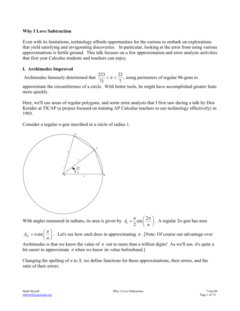
Why I Love Subtraction
Even with its limitations, technology affords opportunities for the curious to embark on explorations
that yield satisfying and invigorating discoveries. In particular, looking at the error from using various
approximations is fertile ground. This talk focuses on a few approximation and error analysis activities
that first year Calculus students and teachers can enjoy.
I. Archimedes Improved
223
22
   , using perimeters of regular 96-gons to
71
7
approximate the circumference of a circle. With better tools, he might have accomplished greater feats
more quickly.
Archimedes famously determined that
Here, we'll use areas of regular polygons, and some error analysis that I first saw during a talk by Don
Kreider at TICAP (a project focused on training AP Calculus teachers to use technology effectively) in
1993.
Consider a regular n-gon inscribed in a circle of radius 1.
D
C
1
1
2
n
...
A
1
B
n  2 
With angles measured in radians, its area is given by An  sin 
 . A regular 2n-gon has area
2  n 
 
A2 n  n sin   . Let's see how each does in approximating  . [Note: Of course our advantage over
n
Archimedes is that we know the value of  out to more than a trillion digits! As we'll see, it's quite a
bit easier to approximate  when we know its value beforehand.]
Changing the spelling of n to X, we define functions for these approximations, their errors, and the
ratio of their errors:
Mark Howell
mhowell@gonzaga.org
Why I Love Subtraction
7-Jun-09
Page 1 of 12
It appears we did four times better using 2n sides compared with n sides. That is,
A2 n   1
 . When
An   4
4 A2 n  An
. Then we can use this information to
3
improve our approximation. Notice that we've also redefined our error functions to use this improved
approximation.
we isolate  in this approximation, we get  
Now it appears we did sixteen times (0.625) better using 2n sides compared with n sides. That is,
A2 n   1
 . That worked so well, let's try to refine our approximation again! [Note: At this point,
An   16
when I tried this on a TI-83, it squawked about an illegal nest. That's why I switched to the HP40gs.
You can get around it on the TI by defining some of the functions explicitly instead of using function
composition, but it gets messy.]
Maybe this is 64 times better. [The alert reader will notice that the table only goes up to X=10. Our
approximation is now so good that we're beginning to exceed the precision of our machine.] One more
time:
We've earned ten digits of accuracy. Amazing!
II. Power Zooming
The next few examples rely on a graphical technique called power zooming that I first saw in the Dick
and Patton Calculus textbook. An explanation of power zooming appears in an appendix of the
Approximation Topic Focus workshop materials for AP Calculus.
Mark Howell
mhowell@gonzaga.org
Why I Love Subtraction
7-Jun-09
Page 2 of 12
III. The Difference Quotient versus the Symmetric Difference Quotient
Subtraction gives insight into a central idea in Calculus, that the limit of the average rate of change of a
function over a closed interval as the width of the interval approaches zero, when it exists, is the
instantaneous rate of change of the function. So, to approximate the derivative of a function f at a
f  a  h  f  a 
point x = a, it suffices to calculate
for values of h that are close to 0. Most graphing
h
calculators that have a function to calculate a numeric derivative don't use this approximation, though.
f a  h  f a  h
Instead the symmetric difference quotient is used,
. Why?
2h
On a side note, caution is needed regardless of which approximation method is used. In particular, at
or near a point where the derivative fails to exist, numerical approximations can give erroneous results.
Try these examples:
The derivative of 1/x at x = 10^-6 should be a large negative number, not 1000001. The derivative of
abs(x) at x = 1/50000 should be 1. And at x = .00001, the slope on the graph of y = arctan(x) is
certainly not 1569.7963. What has happened in each of these cases is that the points x + h and x – h
are on opposite sides of a point where the derivative fails to exist. The slope of the secant line is
therefore not a great approximation of the slope of the tangent line!
Let's take a look at why machines use the symmetric difference quotient instead of the one-sided
difference quotient. Here, we'll use the calculators independent variable, X, to represent the familiar h
in the point-definition of derivative shown above. The procedure here allows for any function to be
used, and any point x = a. In this case, we're looking at the derivative of f  x   sin x at x 
  1
that f     .
3 2

3
Note
The errors for each difference quotient are defined in F4(X) and F5(X). It's instructive for students to
look at these error functions for values of X close to 0.
Mark Howell
mhowell@gonzaga.org
Why I Love Subtraction
7-Jun-09
Page 3 of 12
Zooming in to the table simply divides the increment in the table by the zoom factor. You can do the
same thing on the TI calculators by manually changing the calculator's variable, Tbl. Notice that the
errors in both derivative approximations approach 0 as the h (here, spelled X) approaches 0. Let's look
more closely at how those errors go to zero.
Here's the graph of the error functions in a decimal window:
Now we'll zoom in at the origin with factors of 4x4:
It seems that the one-sided difference quotient's error is straightening out, while the symmetric
difference quotient error is getting flatter. Referring to the aforementioned appendix about power
zooming, this is evidence that the former is behaving like a linear function, while the latter's behavior
is higher degree. To confirm, we'll try to zoom in again, with factors of 4x16 (a degree 2 power
zoom):
This time, the error for the one-sided difference quotient gets steeper, while the shape of the symmetric
difference quotient error remains unchanged. This is evidence that the symmetric difference quotient
error is behaving like a degree two power function. Cool! Higher degree error functions are better
than lower degree because they stay near zero longer. Steep error functions are bad.
Here's another take on this activity from a numeric perspective, using lists on a TI-83/4.
In Y1, we put the function whose derivative we are approximating. In Y2, we have the one-sided
difference quotient approximation for Y1  A , and in Y3 we have the symmetric difference quotient
approximation for Y1  A .
Mark Howell
mhowell@gonzaga.org
Why I Love Subtraction
7-Jun-09
Page 4 of 12
In Y4, we put the exact value of the derivative, Y1  A . Then, in Y5 and Y6, we put the errors from
using the one-sided and the symmetric difference quotient approximations, respectively. Only Y5 and
Y6 are selected.
Store any real number is the variable A (0.5 was chosen for the example here). Then explore this
result numerically by looking at a table of values near X=0.
Note that Y5, the DQ errors, has a constant difference of about .0003, indicating linearity. For Y6, the
SDQ errors, the second differences are constant. Now for some list operations to confirm these results.
Check out the screen shots:
Pretty cool, huh? You can go back and redo this activity with any function in Y1, and with any value
stored in the variable A where Y1 has a derivative. You also need to put the exact derivative value in
Y4. It's needed to get the error. The amazing thing is that it doesn't matter what function you work
with nor what point (unless we're at a point of inflection). Eventually, the error in the SDQ behaves
like a quadratic, and the error in the DQ behaves like a line. Again, we prefer error functions that
behave with a higher degree, since higher degree power functions stay close to zero longer. That's why
the calculators use the symmetric difference quotient.
Mark Howell
mhowell@gonzaga.org
Why I Love Subtraction
7-Jun-09
Page 5 of 12
IV. The Tangent Line as "The Best" Linear Approximation (from Approximation Topic Focus
Materials)
In this activity, you will investigate why the tangent line is called "The Best” linear approximation to a
function at a point. This activity can be done with AB or BC students. Suggested questions to ask
students during the activity appear in italics the narrative. In the figure below, the function
f ( x)  ln( x) is graphed, along with several linear functions that intersect the graph of f at the point (1,
0).
y  x 1
y  .6( x  1)
y  ln  x 
Any of those lines could be used to approximate the value of ln  x  near x = 1. In this activity, we'll
explore how to use linear functions to approximate function values, and why we call the tangent line
"The Best".
Now that we have inexpensive calculators to evaluate transcendental functions, it's harder to justify the
use of tangent lines to approximate function values. Nonetheless, learning how to do so has more
value than just to become familiar with an historic footnote. The tangent line is special for reasons that
penetrate deeply into calculus concepts.
Mark Howell
mhowell@gonzaga.org
Why I Love Subtraction
7-Jun-09
Page 6 of 12
In order to use the tangent line to approximate a function, we must be able to write an equation for that
line. Writing an equation for a tangent line requires that we be able to do two things: determine the
exact function output at a point, and calculate the exact value of the slope at that point. Here we'll use
1
the function f ( x)  ln( x) and the point (1, 0). The derivative is f ( x)  and so f (1)  1 and our
x
tangent line equation is y  x  1 . We'll use the calculator to investigate the tangent line and some
other lines as approximations for ln(x) near x = 1.
First, define functions as shown in the screen below, and take a look at their graphs in the decimal
window:
What would the error be if each line were used to approximate ln(1)? Why?
We'll use the calculator to see how well each line does in approximating ln(2) :
As you can see from the screen shots above, the line through (1, 0) with the wrong slope actually does
a much better job than the tangent line in approximating ln(2)!
Use the second derivative to explain why the line with slope 0.6 does better at approximating ln(2).
From the graph, this isn't surprising. The line in Y3 has a slope that is less than the slope of ln(x) at x =
1. The slope of ln(x) is always decreasing, so it does make sense that at some point, the line with a
slope that is too small will actually do better. In fact, there's even a point where that other line
intersects the graph of y = ln(x) and of course, at that point, its error in approximating ln(x) would be
zero! In order to see why the tangent line is called "The Best", we'll need to look more closely.
Let's define functions that reveal the error in each approximating line. Since our interest is focused
only on the error, be sure to deselect Y1, Y2, and Y3. You might also want to change the graphing
style of the tangent line error, so you can tell it apart from the error of the line with slope 0.6:
Explain why each line passes through the point (1, 0).
Mark Howell
mhowell@gonzaga.org
Why I Love Subtraction
7-Jun-09
Page 7 of 12
Notice that in this decimal view, the error from using the line with slope 0.6 seems to be closer to the
x-axis, indicating that smaller error. What happens if we zoom in at the point of tangency, (1, 0)?
Make sure your zoom factors are equal to start out, and be sure to position the zoom cursor on (1, 0):
Use the second derivative to explain why the tangent line error is always positive.
Zoom in a couple more times:
What happened to the tangent line error as you zoomed in with equal factors?
Notice that as the values of x got closer to 1, the tangent line error flattened out. The error from the
other line, however, though it initially changed shape a bit, as we look closer continues to look linear
and maintain the same steepness. Referring to the results from the appendix on power zooming, these
features indicate that the tangent line error is behaving with a degree greater than 1, while the other line
error is behaving like a degree one (linear) polynomial. To confirm this, go back to the decimal
window, change the zoom factors to do a degree two power zoom (here, we used XFact = 4 and YFact
= 16), and try zooming in again (remember to reposition the cursor at (1, 0)):
What happened to the tangent line error as you zoomed in with a degree two power zoom? What
happened to the other line error?
Stunning! The tangent line error keeps the same shape under a degree two power zoom, while the
other line error gets steeper. Steep error is bad!
Of course, what's special about any tangent line is that its slope agrees with the function at the point of
tangency. You could to repeat this activity with any differentiable function, and the results would be
the same. The error from any line with the wrong slope will behave like a degree one polynomial. At
worst, the tangent line error exhibits degree two behavior. Occasionally, it'll do even better than that.
For example, if you use y = x, the tangent line to f ( x)  sin  x  at x = 0, you'll see that the error
behaves like a degree three power function. This fact is intimately connected with the fact that the
second derivative of sin  x  is 0 at x = 0.
Mark Howell
mhowell@gonzaga.org
Why I Love Subtraction
7-Jun-09
Page 8 of 12
The results of this activity lay the foundation for Taylor Polynomials, a BC-only topic. Let's use a
different function, g  x   e x , and a different point, (0, 1), to explore further.
Since g   x   g   x   e x , g   0   g   0   1 . The tangent line at x = 0 is y = x + 1. You could repeat
the activity above with the functions shown:
Trace over to x = 0.5 on the two error functions, as shown above. You'll see that Y3 actually does a
better job approximating e than Y2 does! As before, we need to look closer to see the difference
between these two linear approximations.
Do a degree two power zoom at the origin, and you should see the same results we saw earlier: the
tangent line error eventually maintains its parabolic shape, while the error in the other line gets steeper.
Now, we'll build a quadratic function to approximate e x near x = 0. To do so, we'll define a quadratic
whose output, slope, and second derivative all match those of e x at x = 0. The quadratic that does the
x2
trick is q( x)   x  1 .
2
Verify that q  0   q  0   1 .
We'll also need a quadratic whose output and slope agree with e x at x = 0, but whose second derivative
x2
 x  1 will work.
is slightly off. The quadratic r ( x) 
1.7
Verify that r(x) has the correct output and slope, but that its second derivative is wrong.
Once again, we'll turn to the calculator to investigate how the error functions behave.
First, check out the errors at x = 0.5. Notice that both quadratics did better than either one of the
tangent lines we looked at above.
Explain why are Y4 and Y5 both go through the origin.
Mark Howell
mhowell@gonzaga.org
Why I Love Subtraction
7-Jun-09
Page 9 of 12
Again, though, the wrong quadratic did a better job! In this case, the second derivative of Y3 is greater
than 1, the second derivative of e x at x = 0. Notice that the third derivative of e x is also 1, and so the
second derivative is increasing. So it isn't altogether surprising that Y3 did better, since its second
derivative is too big. When we look closer, though, we should see the difference between Y2 and Y3.
So, let's try a degree two power zoom at the origin:
The error in the "good" quadratic's error is flattening out under the degree two power zoom, while the
error in the other quadratic is maintaining the same shape.
What do the graphs tell you about the degree of the behavior of the two errors?
This indicates that the degree behavior for the good quadratic is greater than two, while the other
quadratic's error is behaving like a degree two. The natural thing to do is try a degree three power
zoom, and see if the good quadratics error keeps the same shape.
Pretty convincing! The other quadratic's error is getting steeper, while the good quadratic's error is
maintaining its shape.
Understanding the "why" for all of this is relatively straightforward if you look at the Taylor
Polynomials involved. We know, for instance, that the Taylor Polynomial for ln(x) at x = 1 is
 x  1
 x  1

2
 x  1

3
 ... . If we subtract this from the expression for the tangent line at x = 1, x –
2
3
1, the lowest degree we are left with is two.
x 2 x3
  ... . Subtract our "good" quadratic,
2! 3!
x2
x2
 x  1 , and the lowest degree we are left with is three, Subtract the other quadratic,
 x  1 , and
2
1.7
we still have a degree two term. Near where they are zero, the lower degree terms dominate the
behavior.
Similarly, the McLaurin polynomial for e x is 1  x 
Note:
These activities were inspired by a talk by Don Kreider at TICAP in the early 1990's.
Mark Howell
mhowell@gonzaga.org
Why I Love Subtraction
7-Jun-09
Page 10 of 12
V. Errors in Numerical Integration Techniques. Two programs have been prepared to help with
this activity: ACINTERR and INTERR. Each allows you to select a numerical integration method,
and creates lists of data that help analyze errors in the chosen method(s). The first lets you look at
accumulated errors over a wide interval. The second lets you look at errors over each subinterval. To
use the programs, define your integrand in Y1, and an antiderivative for it in Y2. For example, define
Y1(X)=X^3/24 and Y2(X) =X^4/96. Set up the ZDecimal window, then execute the INTERR
program. The program traverses across the currently defined graph screen, evaluating the signed area
over each subinterval on the graph screen by the chosen method.
It uses the Second Fundamental Theorem (with your antiderivative in Y2) to calculate the exact area,
then subtracts these to find the error in each method. The approximated areas are stored in L2. The
errors are stashed away in L3 through L6. If the Left Endpt rule is selected, its errors are stored away
in L3. If the midpoint rule is selected, L4 is used for the errors. If the Right Endpt rule is selected, L5
is used, and if the Trapezoid Rule is selected, L6 is used. L1 always holds the sampled values of the
independent variable. Once you've run through the methods, you can then use the statistics
environment to examine these errors both graphically and numerically!
Here are some screen snapshots using results from INTERR. First, the errors in the left and right
endpoint rules are illustrated:
It appears that the errors have parabolic shape. Remember that the integrand is a cubic. Errors in the
left and right endpoint rules are proportional to the first derivative of the integrand. Now for the errors
in the trapezoid and midpoint rules:
Mark Howell
mhowell@gonzaga.org
Why I Love Subtraction
7-Jun-09
Page 11 of 12
Linear! Proportional to the second derivative! And opposite in sign!
The ACINTERR program does essentially the same thing, but it computes accumulated area as
t3
X min 24 dt for every x across the graph
screen, and then finds the error in the selected method. Here are some screen snapshots:
well as accumulated error. That is, it approximates
X
The output in the middle above is the result of graphing the accumulation function,
t3
X min 24 dt and on
X
the right are the graphs of the left and right endpoint accumulated errors.
On the right above are the errors from the midpoint (positive error) and trapezoid errors. Amazing!
The shape of these errors is striking. It appears that the accumulated left and right endpoint errors are
proportional to the original function, while the midpoint and trapezoid errors are proportional to the
derivative of the original function (a cubic, remember). Why should that be?
This is a graphic view of the motivation behind Simpson's Rule (which, alas, no longer appears in the
AP Calculus Course Description): the trapezoid rule seems to err in the opposite direction from the
midpoint, and the midpoint seems to be about twice as good!
Mark Howell
mhowell@gonzaga.org
Why I Love Subtraction
7-Jun-09
Page 12 of 12