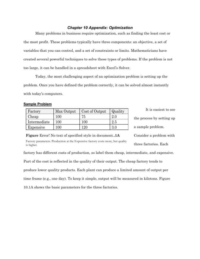
Chapter 10 Appendix: Optimization
Many problems in business require optimization, such as finding the least cost or
the most profit. These problems typically have three components: an objective, a set of
variables that you can control, and a set of constraints or limits. Mathematicians have
created several powerful techniques to solve these types of problems. If the problem is not
too large, it can be handled in a spreadsheet with Excel’s Solver.
Today, the most challenging aspect of an optimization problem is setting up the
problem. Once you have defined the problem correctly, it can be solved almost instantly
with today’s computers.
Sample Problem
Factory
Cheap
Intermediate
Expensive
Max Output
100
100
100
Cost of Output
75
100
120
Quality
2.0
2.5
3.0
It is easiest to see
the process by setting up
a sample problem.
Figure Error! No text of specified style in document..1A
Consider a problem with
Factory parameters. Production at the Expensive factory costs more, but quality
is higher.
three factories. Each
factory has different costs of production, so label them cheap, intermediate, and expensive.
Part of the cost is reflected in the quality of their output. The cheap factory tends to
produce lower quality products. Each plant can produce a limited amount of output per
time frame (e.g., one day). To keep it simple, output will be measured in kilotons. Figure
10.1A shows the basic parameters for the three factories.
Order
Order 1
Order 2
Total Quantity
100
150
Min. Quality
2.5
1.5
Figure Error! No text of specified style in
document..2A
Order specifications. You will have to mix output from the
three factories to provide the desired quantity and quality.
Now, say that two orders arrive
that both need to be filled over the
same time period. The details of the
orders are shown in Figure 10.2A. To
meet the quantity and quality
specifications, you will have to mix output from the three factories. The ultimate question
is: What is the cheapest way of allocating production from each factory to fill the two
orders?
Problem Definition
This problem is an
Variables: things you can control
Output from each factory (c, i, e) given to each order (1, 2):
Qc1, Qi1, Qe1, Qc2, Qi2, Qe2
Goal: objective function
Minimize total cost:
Cost = 75 Qc1 + 75 Qc2 + 100 Qi1 + 100 Qi2 + 120 Qe1 + 120 Qe2
Constraints: restrictions or limits
Plant Limit C:
Plant Limit I:
Plant Limit E:
Quantity Order 1:
Quantity Order 2:
Quality Order 1:
Quality Order 2:
Qc1 + Qc2 <= 100
Qi1 + Qi2 <= 100
Qe1 + Qe2 <= 100
Qc1 + Qi1 + Qe1 = 100
Qc2 + Qi2 + Qe2 = 100
2.0 Qc1 + 2.5 Qi1 + 3.0 Qe1 > 250 (2.5 * 100)
2.0 Qc2 + 2.5 Qi2 + 3.0 Qe2 > 225 (1.5 * 150)
Figure Error! No text of specified style in document..3A
Problem definition. Note the six variables that we need to solve. The goal is
to minimize total cost. The answer must meet the constraints on the plants
and on the orders.
optimization problem
because the goal is to choose
output variables that
produce the least cost
solution. The problem
contains several constraints
in the form of limits on
production and specifications
for the order. The basic
description of the problem is shown in Figure 10.3A. The most important step in setting up
the problem is to realize there are six control variables contained in the amount of
production from each plant that is given to each order.
Spreadsheet Layout
=C3*C2+D3*D2+E3*E2+F3*F2+G3*G2+H3*H2
=C4*C2+D4*D2
Variables Qc1
Qc2
Qi1
Qi2
Qe1
Qe2
Limit
Constraint
Objective
Plant C limit
Plant I limit
Plant E limit
Order 1
Order 2
Quality Order 1
Quality Order 2
0
75
1
75
1
1
100
100
1
1
1
1
2.5
2
120
1
1
1
2
120
1
1
3
2.5
3
0
0
0
0
0
0
0
<=
<=
<=
=
=
>
>
100
100
100
100
150
250
225
Figure Error! No text of specified style in document..4A
Spreadsheet layout. Put each control variable (Qc1, Qc2, … Qe2) in a column. Put the objective function
parameters in a row. Define each constraint in a row, where the total is compared to a limit value.
Some optimization systems enable you to enter the problem definition as it is
written in Figure 10.3A. However, if you want to use Excel’s Solver for the problem, it is
easier to first lay out the problem in the spreadsheet. This step makes it easier to change
values later and examine the effects of changes.
As shown in Figure 10.4A, you want to define a column for each of the control
variables. Leave a blank cell (row) that will hold the actual value (solution) for each
variable. Then put the parameters for the objective function on a new row. Finally, create
rows for each of the constraints. Each constraint has parameter values that will be
multiplied by the variable and summed for each row. This total is compared to the limit
value.
Start with the objective function. You must define a cell that contains the total cost
value (which will be minimized). Multiply each cost parameter by the amount that will be
produced and compute the total. For example, 75*Qc1 + 75*Qc2 + 100Qi1 and so on. Each
parameter (75) and variable (Qc1) is defined by the appropriate cell (e.g., C3*C2 + D3*D2).
Currently the total is zero because there is no solution yet and all of the quantities are zero.
Define the constraints similarly. For instance, for factory C, add the amount
produced for order one (1*Qc1) to that produced for order two (1*Qc2). This total must be
less than or equal to the capacity of factory C (100). On the plant C row, you put a 1 in the
columns for Qc1 and Qc2. Then you enter the value 100 in the limit column. In the
constraint column, you enter a formula to add: 1*Qc1 + 1*Qc2 + 0*Qi1 and so on. The other
constraints are defined just as easily.
Excel Solver
Variables Qc1
Qc2
Qi1
Qi2
Qe1
Qe2
Limit
Constraint
Objective
Plant C limit
Plant I limit
Plant E limit
Order 1
Order 2
Quality Order 1
Quality Order 2
0
75
1
75
1
1
100
100
1
1
1
1
1
1
2
1
2.5
2
120
120
1
1
3
2.5
3
0
0
0
0
0
0
0
<=
<=
<=
=
=
>
>
100
100
100
100
150
250
225
Figure Error! No text of specified style in document..5A
Excel Solver. You need to tell the Solver where to find the three elements: objective function
total, control variables, and the constraints.
The next step is to start the Excel Solver and tell it where to find the three
components (control variables, objective function, and constraints). Figure 10.5A shows the
basic form for the Solver. Use the total value for the objective function as the target cell.
The “changing cells” are the control variable cells that you set aside earlier.
You must add each constraint separately. When you click the Add button, enter the
cell for the computed value (the constraint column), choose the appropriate inequality or
equality sign, then set the cell for the limit value. Technically, you could enter the
inequality similar to the way it is shown in Figure 10.3A; however, it is better to use the
method shown in Figure 10.5A. That way it is easy to change the constraint parameters
and the limit values. Entering new values in the spreadsheet is much easier than editing
the inequality in the Solver.
Solution
Variables Qc1
Qc2
Qi1
Qi2
Qe1
Qe2
28.555 71.445 41.327 58.673 30.118 19.882 Constraint
Objective
23500
75
75
100
100
120
120
Plant C limit
1
1
100 <=
Plant I limit
1
1
100 <=
Plant E limit
1
1
50 <=
Order 1
1
1
1
100 =
Order 2
1
1
1
150 =
Quality Order 1
2
2.5
3
250.7813 >
Quality Order 2
2
2.5
3 349.2188 >
Limit
100
100
100
100
150
250
225
Figure Error! No text of specified style in document..6A
Solution. The Solver fills in the values for the control variables (28.555 to 19.882). The spreadsheet then
computes the total cost and the value of each of the constraints. Notice that each constraint is satisfied,
indicating
a feasible
Once
you solution.
have the three components entered, you simply click the Solve button. The
Solver will tell you if it finds an acceptable solution. If not, you probably have infeasible
constraints and you should double-check all of the constraints. If necessary, start with a
simpler problem with few constraints; then add constraints until you find the problem. In
some cases, there might not be a feasible solution. For example, what would happen if the
two orders required a total of 450 kilotons? This problem could not be solved because the
total output of the three plants is only 300.
The solution to the sample problem is shown in Figure 10.6A. The Solver fills in the
control values for the solution. The spreadsheet then computes the total cost and the value
for each constraint. Notice that because all the constraints are satisfied, the solution is
feasible. Also note that the expensive plant is used to produce only 50 kilotons. Remember
that the total plant capacity was 300, and the total of the two orders was only 250. Hence,
the solution makes sense because the slack is at the most expensive factory.
What happens if costs change, or if the customers change their quality
specifications? You simply change the parameters in the spreadsheet, restart the Solver,
and click the Solve button.
Limitations
One issue you might encounter is a limit on the number of variables or constraints.
The actual limits within the Excel Solver change with new versions, but it is unlikely that
it will be able to handle problems with more than a couple hundred variables and
constraints.
If you look carefully at the sample problem in Figure 10.3A, you will notice that the
objective function and the constraints are all linear. For example, there are no quadratic or
other nonlinear terms. These types of problems are relatively easy to solve. On the other
hand, if you have nonlinear constraints, the problem is considerably more difficult to solve.
Although the Excel Solver can handle some degree of nonlinearity, it will probably not work
on complex problems.
In these situations, you will have to find dedicated optimization software to handle
your problem. Fortunately, several commercial software packages can handle very large,
complex optimization problems.
Summary
The power of optimization is that it can identify a precise solution. You do not have
to rely on rules of thumb or guesswork. In many cases, even a seemingly small change can
result in saving thousands or millions of dollars. For instance, AT&T improved their
switching network by embedding an optimization routine that determines the best method
to route phone calls.
Exercises
1. Build the spreadsheet to solve the problem in the text. Test it to see that you get the
correct answer. Now, change the quantity in order 1 to 125 and the quality in order 2 to
1.75. What are the new production values?
2. Identify three business problems (that are not used in this book) that would benefit
from mathematical programming tools.
3. A company wishes to develop new software that is estimated to require 30,000 elements
(e.g., lines of code). It can hire full-time staff who can create 15 elements per day; part
time workers who produce 10 elements a day, or contract with an outside company to
produce 25 elements a day. Full-time workers cost $200 per day, part timers $160 per
day, and contract workers $400 per day. Because of a hiring freeze, the project cannot
use more than 1,000 days of full-time employees (e.g., 3 employees for a year). However,
because of management involvement, at least 500 days of full-time work is required.
The directors are tired of paying for contractors so they will not authorize spending
more than $180,000 on contractors. How many days of full-time, part-time, and contract
work is needed to minimize costs?