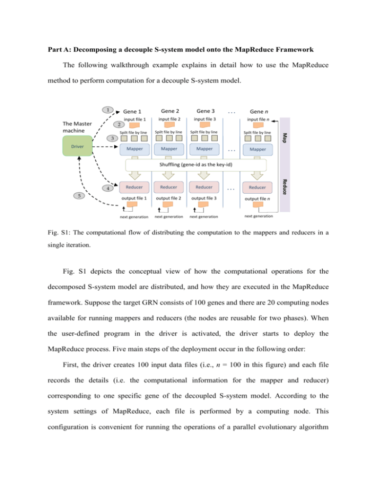
Part A: Decomposing a decouple S-system model onto the MapReduce Framework
The following walkthrough example explains in detail how to use the MapReduce
method to perform computation for a decouple S-system model.
1
Gene 1
2
Spilt file by line
Gene 2
Gene 3
input file 2
input file 3
input file n
Spilt file by line
Spilt file by line
Spilt file by line
Mapper
Mapper
...
Gene n
3
Driver
Mapper
...
Map
The Master
machine
input file 1
Mapper
Shuffling (gene-id as the key-id)
5
Reducer
Reducer
Reducer
output file 1
output file 2
output file 3
next generation
next generation
next generation
...
Reducer
Reduce
4
output file n
next generation
Fig. S1: The computational flow of distributing the computation to the mappers and reducers in a
single iteration.
Fig. S1 depicts the conceptual view of how the computational operations for the
decomposed S-system model are distributed, and how they are executed in the MapReduce
framework. Suppose the target GRN consists of 100 genes and there are 20 computing nodes
available for running mappers and reducers (the nodes are reusable for two phases). When
the user-defined program in the driver is activated, the driver starts to deploy the
MapReduce process. Five main steps of the deployment occur in the following order:
First, the driver creates 100 input data files (i.e., n = 100 in this figure) and each file
records the details (i.e. the computational information for the mapper and reducer)
corresponding to one specific gene of the decoupled S-system model. According to the
system settings of MapReduce, each file is performed by a computing node. This
configuration is convenient for running the operations of a parallel evolutionary algorithm
(EA).
Second, the driver then dispatches a number of job tasks to the mapper nodes. In this
example, there are 100 genes to be inferred. Therefore, each node is responsible for 5 map
tasks. Note that if the size of a single file exceeds the maximum memory capacity, e.g. 64
MB, the file will be divided into smaller tasks. In our application case, one file corresponds
to a map task.
Third, a mapper node reads the file and divides the file line by line. Each line has a
string format that contains all the information to be utilized for the parallel EA. The line
(string) is regarded as the basic unit for a specific gene of the S-system model. After
performing some computation specified by the user-defined program (e.g. the EA
operations), a mapper saves the results in the local memory and sets gene-id as the key-id to
be used by the reducer in the next step. The concept of using the key-id in MapReduce is
that all information corresponding to a target gene is identified by the given key-id, so the
key-id can be used by the reducers to retrieve the information of a specific gene. The results
corresponding with the same key-id are then collected for the same reducer.
Fourth, once the computing nodes are idle, they become the reducer nodes. After a
reducer groups the operations related to a specific gene, it starts to execute the user-defined
program and output the results corresponding to the key value. Then, the reducer will
continue to group the operations for the next key-id until output for all key-ids (i.e., gene-ids)
have been produced in the reduce phase.
Fifth, the driver continues to designate job tasks for mapper nodes, if the above process
needs to be performed iteratively. If not, the driver will summarize the final result of the
complete model. In this example, the inferred results for the 100 genes are aggregated by the
reducer.
In the process mentioned above, MapReduce takes care of almost all of the low-level
details, including the data distribution, communication, fault tolerance, etc. one can
therefore concentrate on the algorithms and define the map/reduce methods. Specifically
speaking, the user only has to design four objects, which are categorized into two types of
computational functions: map and reduce phases. The first two objects are for the map phase,
including a map method and the input format with respect to the key-id/value pair per record
that would be read and processed by the map method. Here, the key-id represents one
individual gene in the S-system model and the value along with a key-id records the
information for the user-defined computational operations, such as the parameters used in
the parallel EA. The remaining two objects for the reduce phase include a reduce method
and the output format that will be transformed into output records.
Part B: Control flow and data format
The operational flow of the MapReduce model can be described in detail as follows
(see Fig. 4 of the manuscript). The driver module in the master machine is responsible for
the iteration control of the iGA-PSO computation performed by the slaves. In other words,
every iGA-PSO iteration starts a dispatching process once to distribute the relevant
operations into the map and reduce phases for computation. The driver also sends the input
document to the HDFS files database at the beginning and produces the overall output file
from the HDFS at the end of the run. Specifically, in the Hadoop environment, the
MapReduce process is initialized by the driver, which generates a “Job” and sends it to the
Job Tracker. The Scheduler within the Job Tracker then produces two types of subtasks:
MapTask and ReduceTask (to be executed in the mapper and reducer, respectively) and
dispatches them to the slave machines. The iterative flow is achieved by the driver to create
a new Job and repeat the above procedure.
Before sending a Job to the Job Tracker, the driver must create a Configuration object
to store the parameter settings in HDFS (such as the particle number, the weights for
updating the particle velocity, the migration rate, and so on). These parameters are saved in
the HDFS folders and are shared between the mapper and reducer to ensure data correctness
during the algorithmic computation. Because some parameter values (such as the weight of
each particle) will be changed in each iteration and the computation results conducted in the
mapper or reducer are subject to those values, the driver must designate the Configuration
for each new Job. In this way, a newly created Job can conveniently read the parameters
from the files, and the iGA-PSO code in the mapper and reducer phases can directly use the
parameters to perform the corresponding computation afterwards.
Between the map and reduce phases, the data are shuffled (parallel sorted/exchanged
between computational nodes). The shuffling mechanism groups the particles together
according to which genes they are addressing (by using the gene-id as the key). In this way,
all of the particles that correspond to a given key end up at the same reducer to perform the
remaining operations that must rely on the results produced by others. Here, using gene-id as
the key in shuffling can keep the particle distribution uniform and thus alleviate the problem
of becoming overloaded. This problem often occurs in the implementation of
evolution-based algorithms with the MapReduce model. It is caused by a situation in which
the algorithm proceeds (converges), the same (close to optimal) individual starts to dominate
the population, and all copies of this individual are sent to a single reducer. In other words,
the distribution of the computation becomes unbalanced, and the efficiency of the
parallelism decreases as the algorithm converges. As a result, the algorithm will require
more iterations to derive the final solution.
As can be observed from the data format used in the proposed approach (see Fig. 5 in
the paper), the particles play central roles in conducting the computation. Specifically, at
each MapReduce stage (iteration), we create a data string for each particle so that the
Hadoop environment can handle the overall computational workflow smoothly. In this study,
as mentioned in the paper, the data recorded in the string is categorized into two types. The
first type of data is defined as the identifiers for the shuffling procedure; i.e., gene-id,
island-id, and particle-id, which indicate the gene that a particle is addressing, the group that
the particle belongs to, and the performance rank of the particle, respectively. The second
type of data is defined to indicate the particle states; i.e., the position, velocity, and fitness,
the pbest-position of this particle, and the gbest-position of the swarm.
With the above settings for control flows and data format, the driver module can
control the two parts of the iGA-PSO without continuing to read the HDFS iteratively (as
shown in Fig. 4 of the manuscript). This goal is achieved through the procedure of
periodically updating the Job’s input/output paths (files) recorded in the HDFS. After the
MapReduce process has been performed once, the driver changes the path of the input file to
be that of the output file, to use the computational results that were obtained from the
previous iteration. The driver simply passes the corresponding path to a mapper to perform
the relevant computation; and, thus, saves much of the I/O effort by only writing/reading the
HDFS at the first/final iteration.
Part C: Using structural knowledge in network inference
To demonstrate how the structural knowledge can improve the correctness of the network
topology, we use two different fitness functions to conduct a set of experiments for
comparison: the original MSE function, and the other fitness function. The new fitness
function includes two major parts as follows:
f obj (i )    MSE (i )  (1   )  StrEval (i ), for i  1, 2, 3, ..., N
The first part, MSE(i), is used to derive the correct network behavior, whereas the second
part, StrEval(i), is used to maximize the structural accuracy that measures the difference
between the structure suggested by the pre-defined real positive and negative outcomes and
that of the inferred model. The weighting factor α is used to decide the importance of the
two issues to be considered (i.e., the gene expression profiles and the network structure). In
the above function, there are two sub-terms included in StrEval(i), sensitivity and specificity,
as described below.
StrEval (i )  sensitivity (i )  specifictity (i )
The two sub-terms are ratios of the binary classification result. In this equation,
sensitivity(i)  [0, 1] is the true positive rate. It indicates how many kinetic orders belonging
to gene i follow the suggestion that a plausible connection (a true positive connection)
should exist between gene i and other genes j. In contrast, specificity  [0, 1] is the value of
the true negative rate, which means how many kinetic orders belonged to gene i are negative
connections.
The above two fitness functions were used to infer the network model from the dataset 1
described in the paper (i.e., the 25 nodes dataset). Table S1 depicts the result of the structural
classification for using the original MSE function; table S2 is the result of adopting the
fitness function with structural information. As shown in the two tables, the fitness function
considering both the expression error and structural information outperforms the MSE
function, in terms of the precision and recall rates. That is, 18.44% versus 51.38% for the
precision rate, and 90.17% versus 97.11% for the recall rate, respectively.
Table S1. The structural classification matrix for dataset 1 (25 nodes) evaluated by the original
fitness function.
Actual Class
Connection
Predicted
Class
No connection
Connection
No connection
156
690
Positive predictive rate
(true positive)
(false negative)
(precision): 18.44%
17
387
Negative predictive rate:
(false positive)
(true negative)
95.79%
Sensitivity (recall):
Specificity:
Total Accuracy:
90.17%
35.93%
43.33%
Table S2. The structural classification matrix for dataset 1 (25 nodes) evaluated by the proposed
fitness function.
Actual Class
Connection
Predicted
Class
No connection
Connection
No connection
168
159
Positive predictive rate
(true positive)
(false negative)
(precision): 51.38%
5
918
Negative predictive rate:
(false positive)
(true negative)
99.46%
Sensitivity (recall):
Specificity:
Total Accuracy:
97.11%
85.24%
86.88%