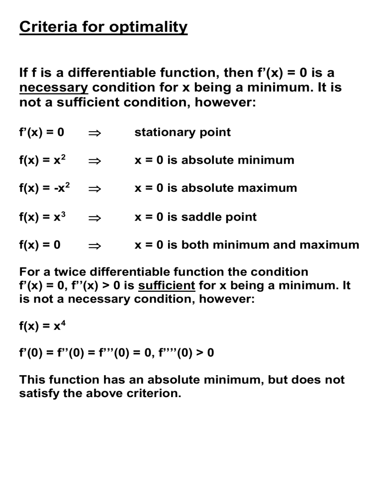
If f is a differentiable function, then f’(x) = 0 is a necessary condition for x being a minimum. It is not a sufficient condition, however: f’(x) = 0  stationary point f(x) = x 2 f(x) = -x 2
 x = 0 is absolute minimum
 x = 0 is absolute maximum f(x) = x 3
 x = 0 is saddle point f(x) = 0
 x = 0 is both minimum and maximum
For a twice differentiable function the condition f’(x) = 0, f’’(x) > 0 is sufficient for x being a minimum. It is not a necessary condition, however: f(x) = x 4 f’(0) = f’’(0) = f’’’(0) = 0, f’’’’(0) > 0
This function has an absolute minimum, but does not satisfy the above criterion.

For 2k times differentiable functions, a sufficient criterion is: f’(x) = f’’(x) = … = f (2k-1) (x) = 0, f (2k) (x) >0
Is this also necessary for an infinitely differentiable function, i.e., does a non-zero function that has a minimum, satisfy this criterion for some k?
The answer is: no! Consider f(x) = exp(-1/x 2 ) (if x

0), and f(0) = 0

This function is continuous, infinitely many times differentiable, and f (j) (0) = 0 for all j, but f has an absolute minimum in x = 0.
This function is not analytic in x = 0 (the Taylor series expansion does not converge to the function).
Generalization to higher dimensions: f:R n 
R has a strict minimum in x if
 f(x) = 0 and

2 f(x) > 0

2 f(x) > 0 means that the Hessian matrix of f is strictly positive definite (This means that (

2 f(x)y, y) > 0 for all y

0)
Example1: consider f
 x
1
, x
2
, x
3
  x
1
2
 x
1 x
2
 x
2
2
 x
3
2 . The first and second derivatives are:
 f
 x
1
, x
2
, x
3

 

2 x
1 x
1


2 x
3 x
2
2 x
2


,

2 f
 x
1
, x
2
, x
3

 




2
1
0
1
2
0
0
0
2





The eigenvalues of the Hessian matrix are 1, 2, 3. These are all non-negative, so (0, 0, 0) is a strict minimum.

Example 2: consider f
 x
1
, x
2
, x
3

 x
1
2 x
2
 x
3
2
for x
2
> 0.
The first and second derivatives are:
 f
 x
1
, x
2
, x
3











2
 x
1 x
2 x
1
2 x
2
2
2 x
3









,

2 f
 x
1
, x
2
, x
3










2 x
2
2 x
1
0 x
2
2

2 x x
2
2
2 x
1
2
1 x
3
2
0
0
0
2






 x
1
2

The eigenvalues of the Hessian matrix are 0, 2, 2
3 x
2 x
2
2
.
These are all non-negative, so the matrix is nonnegative definite and the function f is convex. This also follows from the definition of non-negative definite:
2







 y
1 y
2 y
3



,






 x
2
2
0 x
1 x
2
2

2 x x
2
2
2 x
1
2
1 x
2
3
0
0
0
2








 y
1 y
2 y
3









2 x
2

 y
1
 x
1 y
2 x
2


2

2 y
3
2 
0 .
All points (0, x
2
, 0) with x
2
> 0 are (non-strict) minima.

Multivariable unconstrained optimization (Ch 12.5)
Steepest descent method.
The idea of this method is that from a starting point a minimum is found in a steep(est) descent direction.
From that point a new point is then found.
The steepest ascent direction is given by the gradient:
 f(x) = f’(x) T , because from the Taylor approximation f(x+h) = f(x) +
 f(x) T h + O(|h| 2 ). it is clear that
 f(x) is the direction in which f locally increases maximally.
The steepest ascent algorithm works as follows:
0. Find a starting point x
0
1. Find the value t* for which t
 f(x k
+ tf’(x k
)) is maximal
2. x k+1
:= x k
+ t* f’(x k
)
3. If the stopping criterion is satisfied, stop, else k:=k+1 and go to 1

Example: f(x
1
, x
2
) = 2x
1 x
2
+ 2x
2
– x
1
2 – 2x
2
2 f’(x
1
, x
2
) = (2x
2
– 2x
1
2x
1
+ 2 – 4x
2
)
Starting point X
0
= (0,0)
Iteration 1 : f’(0,0) = (0,2)
Find the maximum of f((0,0) + t(0,2)) = f(0, 2t) = 4t – 8t 2 : t* = ¼
X
1
= (0,0) + ¼(0,2) = (0,1/2)
Iteration 2 : f’(0,1/2) = (1 0)
Find the maximum of f((0,1/2) + t(1,0)) = f(t, 1/2) = ½ + t – t 2 : t* = 1/2
X
2
= (0,1/2) + 1/2(1,0) = (1/2,1/2)