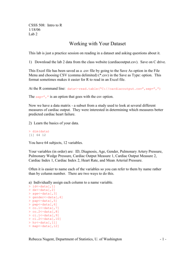
CSSS 508: Intro to R
1/18/06
Lab 2
Working with Your Dataset
This lab is just a practice session on reading in a dataset and asking questions about it.
1) Download the lab 2 data from the class website (cardiacoutput.csv). Save on C drive.
This Excel file has been saved as a .csv file by going to the Save As option in the File
Menu and choosing CSV (comma delimited) (*.csv) in the Save as Type: option. This
format sometimes makes it easier for R to read in an Excel file.
At the R command line: data<-read.table(“C://cardiacoutput.csv”,sep=”,”)
The sep=”,” is an option that goes with the csv option.
Now we have a data matrix - a subset from a study used to look at several different
measures of cardiac output. They were interested in determining which measures better
predicted cardiac heart failure.
2) Learn the basics of your data.
> dim(data)
[1] 64 12
You have 64 subjects, 12 variables.
Your variables (in order) are: ID, Diagnosis, Age, Gender, Pulmonary Artery Pressure,
Pulmonary Wedge Pressure, Cardiac Output Measure 1, Cardiac Output Measure 2,
Cardiac Index 1, Cardiac Index 2, Heart Rate, and Mean Arterial Pressure.
Often it is easier to name each of the variables so you can refer to them by name rather
than by column number. There are two ways to do this.
a) Individually assign each column to a name variable.
>
>
>
>
>
>
>
>
>
>
>
>
id<-data[,1]
dx<-data[,2]
age<-data[,3]
gender<-data[,4]
pap<-data[,5]
pwp<-data[,6]
co.1<-data[,7]
co.2<-data[,8]
ci.1<-data[,9]
ci.2<-data[,10]
hr<-data[,11]
map<-data[,12]
Rebecca Nugent, Department of Statistics, U. of Washington
-1-
b) Define a data frame where each column has a name.
> data<data.frame(id=data[,1],dx=data[,2],age=data[,3],gender=data[,4],pap=dat
a[,5],pwp=data[,6],co.1=data[,7],co.2=data[,8],ci.1=data[,9],ci.2=data[
,10],hr=data[,11],map=data[,12])
Now when you need to access a variable, you can just type: data$age.
It’s always a good idea to take a look at your individual variables to get an overall
picture. One command that will give you the range, mean, median, etc as well as if there
are any missing values is: summary( ).
> summary(dx)
CHF HTx
22 42
> summary(age)
Min. 1st Qu. Median
25.00
54.00
60.00
> summary(data$gender)
f m
4 60
> summary(data$pap)
Min. 1st Qu. Median
11.0
18.0
22.0
> summary(pwp)
Min. 1st Qu. Median
6.10
13.05
16.30
> summary(co.1)
Min. 1st Qu. Median
2.700
4.200
5.200
> summary(co.2)
Min. 1st Qu. Median
1.700
4.300
5.550
> summary(ci.1)
Min. 1st Qu. Median
1.400
2.236
2.600
> summary(ci.2)
Min. 1st Qu. Median
1.000
2.175
2.700
> summary(hr)
Min. 1st Qu. Median
54.00
78.00
85.50
> summary(map)
Min. 1st Qu. Median
76.0
94.0
110.0
Mean 3rd Qu.
57.19
68.00
Max.
80.00
Mean 3rd Qu.
23.9
27.5
Max.
46.0
NA's
5.0
Mean 3rd Qu.
18.50
19.25
Max.
47.40
NA's
5.00
Mean 3rd Qu.
5.347
6.225
Max.
9.700
Mean 3rd Qu.
5.623
7.225
Max.
9.300
Mean 3rd Qu.
2.696
3.063
Max.
5.100
Mean 3rd Qu.
2.787
3.525
Max.
4.600
Mean 3rd Qu.
87.88
98.00
Max.
121.00
Mean 3rd Qu.
109.4
123.0
Max.
145.0
Rebecca Nugent, Department of Statistics, U. of Washington
NA's
2.0
-2-
So who’s missing data?
> which(is.na(pap))
[1] 1 31 47 56 57
> which(is.na(pwp))
[1] 31 47 54 56 57
> which(is.na(map))
[1] 12 64
Note that some people are missing more than one value. So the number of people who
are missing data is NOT found by adding up the number of NA’s for each variable.
> c(which(is.na(pap)),which(is.na(pwp)),which(is.na(map)))
[1] 1 31 47 56 57 31 47 54 56 57 12 64
> unique(c(which(is.na(pap)),which(is.na(pwp)),which(is.na(map))))
[1] 1 31 47 56 57 54 12 64
>
sort(unique(c(which(is.na(pap)),which(is.na(pwp)),which(is.na(map)))))
[1] 1 12 31 47 54 56 57 64
(The unique( ) function removes all duplicates from a vector.)
We can choose subsets of the data matrix by values of just one variable.
Let’s say we want to split up the dataset into males and females.
> females<-data[gender=="f",]
> dim(females)
[1] 4 12
> males<-data[gender=="m",]
> dim(males)
[1] 60 12
Or choose the subset of people who are NOT missing data:
> missing<sort(unique(c(which(is.na(pap)),which(is.na(pwp)),which(is.na(map)))))
> newdata<-data[-missing,]
> dim(newdata)
[1] 56 12
Or a random sample of people from our matrix:
> random.sample<-sample(seq(1,nrow(data)),10)
> random.sample
[1] 52 2 25 54 27 8 40 11 49 17
> sample.subset<-data[random.sample,]
> dim(sample.subset)
[1] 10 12
Can also do any combination of variables:
> data[gender=="m"&age<30,]
(males who are younger than 30)
> data[co.1<4&co.2<4,]
(subjects with both cardiac output measures < 4)
Rebecca Nugent, Department of Statistics, U. of Washington
-3-
We can also select a group of variables (instead of patients).
> new.vars<-cbind(gender,age,dx)
> dim(new.vars)
[1] 64 3
Or
> newvars<-data[,c(4,3,2)]
Practice several conditional statements with this dataset. What are some questions you
would ask about your data?
How many people are older than 45?
> sum(age>45)
[1] 52
What percent of the patients have a mean arterial pressure between 95 and 125?
> sum(map>95 & map<125)/nrow(data)
[1] NA
We have missing data in the map variable.
> sum(!is.na(map)&map>95 & map<125)/nrow(data)
[1] 0.5
If is.na(map) gives you which ones are missing, !is.na(map) gives which ones are not
missing. Putting a ! in front of the true/false commands flips them. Think of the ! as the
putting a not with the command: !is.na = is not missing
Other helpful commands:
any( )
all( )
: checks if there are any trues in your logical vector: returns TRUE or FALSE
: checks if all values are trues in your logical vector: returns TRUE or FALSE
Are there any women in the study?
> any(gender=="f")
[1] TRUE
Are there any missing values in pulmonary wedge pressure?
> all(!is.na(pwp))
[1] FALSE
These are helpful if you have a really long list of true/falses that you don’t want to scan.
Rebecca Nugent, Department of Statistics, U. of Washington
-4-