Practical 3
advertisement
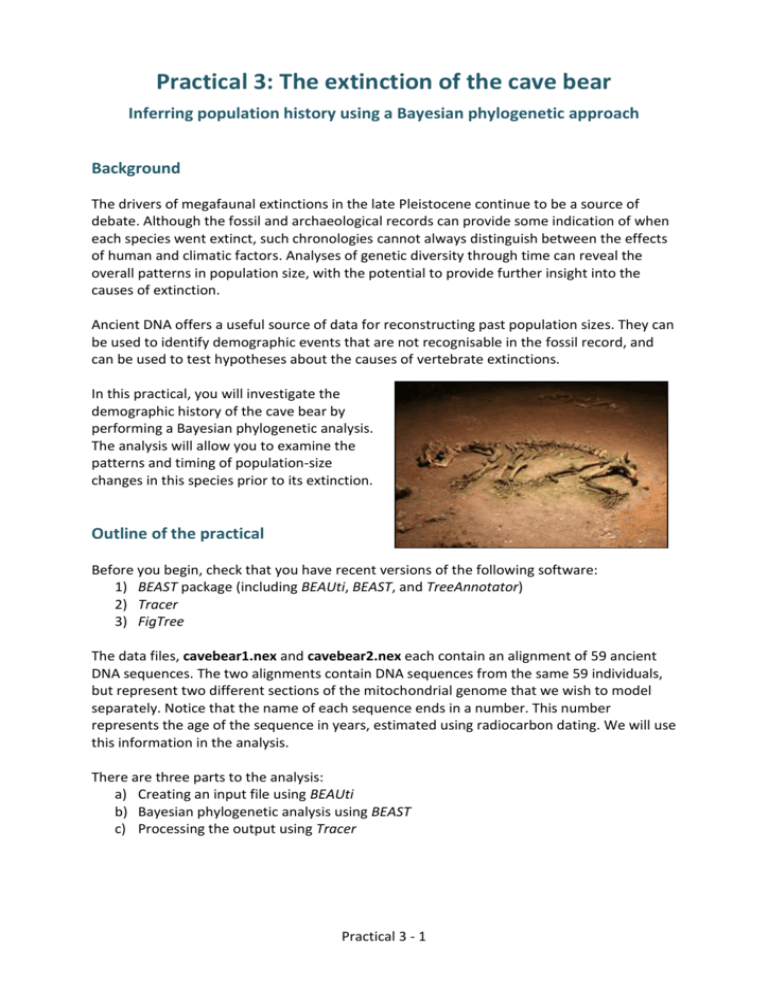
Practical 3: The extinction of the cave bear Inferring population history using a Bayesian phylogenetic approach Background The drivers of megafaunal extinctions in the late Pleistocene continue to be a source of debate. Although the fossil and archaeological records can provide some indication of when each species went extinct, such chronologies cannot always distinguish between the effects of human and climatic factors. Analyses of genetic diversity through time can reveal the overall patterns in population size, with the potential to provide further insight into the causes of extinction. Ancient DNA offers a useful source of data for reconstructing past population sizes. They can be used to identify demographic events that are not recognisable in the fossil record, and can be used to test hypotheses about the causes of vertebrate extinctions. In this practical, you will investigate the demographic history of the cave bear by performing a Bayesian phylogenetic analysis. The analysis will allow you to examine the patterns and timing of population-size changes in this species prior to its extinction. Outline of the practical Before you begin, check that you have recent versions of the following software: 1) BEAST package (including BEAUti, BEAST, and TreeAnnotator) 2) Tracer 3) FigTree The data files, cavebear1.nex and cavebear2.nex each contain an alignment of 59 ancient DNA sequences. The two alignments contain DNA sequences from the same 59 individuals, but represent two different sections of the mitochondrial genome that we wish to model separately. Notice that the name of each sequence ends in a number. This number represents the age of the sequence in years, estimated using radiocarbon dating. We will use this information in the analysis. There are three parts to the analysis: a) Creating an input file using BEAUti b) Bayesian phylogenetic analysis using BEAST c) Processing the output using Tracer Practical 3 - 1 Bayesian phylogenetic analysis At this stage you might wish to test your understanding of Bayesian phylogenetics. In maximum-parsimony analysis, we aim to find the most parsimonious tree, which is the tree that requires the fewest steps to explain the data set. In maximum-likelihood analysis, we aim for maximum-likelihood estimates of the parameters and search for the maximumlikelihood tree. In a Bayesian framework, we regard all parameters as having distributions. Our goal is to estimate the posterior distributions of parameters of interest. The posterior distributions represent the combination of the prior distributions (specified by the user) and the likelihood (calculated from the data). In other words, posterior prior x likelihood. Q. How do we choose the prior distribution for each parameter in the analysis? ......................................................................... ......................................................................... Q. Would it be appropriate to use estimates from our data set to inform our choice of prior distributions? Why or why not? ......................................................................... ......................................................................... ......................................................................... Q. Given that it is not possible to estimate the posterior distribution directly, what method can we use to gain an approximation of the posterior distribution? ......................................................................... Q. In maximum likelihood, we can gain an idea of the uncertainty in an estimate by constructing a 95% confidence interval. What is the Bayesian counterpart to a ‘95% confidence interval’? ......................................................................... Q. In terms of estimating support for nodes in the inferred phylogeny, what is the advantage of using a Bayesian approach compared with maximum likelihood? ......................................................................... ......................................................................... ......................................................................... ......................................................................... Practical 3 - 2 Part A: Creating an input file using BEAUti a) Open the program BEAUti. The purpose of this software is to create a working input file for Bayesian phylogenetic analysis using BEAST. The first step is to load the sequence data into the program. Select “Import Alignment” from the “File” menu and open the alignment files, cavebear1.nex and cavebear2.nex. b) You should now be in the Partitions section of BEAUti. The window will display some of the characteristics of the data that you have loaded. We can see two alignments, each containing 144 nucleotide sites from 59 individuals. We want to model each of these alignments separately and allow the two mitochondrial regions to have different mutation rates. To do this, select both of the alignments, then click on “Unlink Subst. Models” and “Unlink Clock Models”. This means that we are allowing the two regions to have separate substitution models and separate clock models. However, we want the two regions to have the same tree model. Both regions are from the mitochondrial genome and so they are completely linked. Q. Why does unlinking the substitution models increase the number of parameters in the analysis? ......................................................................... ......................................................................... ......................................................................... Q. In what situation might we wish to unlink the trees for different parts of the alignment? ......................................................................... ......................................................................... ......................................................................... ......................................................................... c) Skip the Taxon Sets section. d) Go to the Tips section. Here we will use the ages of the sequences, obtained via radiocarbon dating, to calibrate our estimates of rates and coalescence times. Check the box next to “Use tip dates”. Here we will use the radiocarbon dates that have been included in the sequence names. Click on “Guess Dates”. Select “Defined just by its order”, then select “last” from the drop-down menu next to “Order”. BEAUti will interpret the last field in each sequence name as representing the age of the sequence. In the second drop-down menu next to “Dates specified as”, select “Before the present”. We are choosing this because the dates are given as the number of years before the present day. You will see that the columns “Date” and “Height” have been populated with numbers. The numbers in “Height” denote the age of each sequence, relative to the youngest sequence. Practical 3 - 3 Q. What is the youngest sequence in the data set, and what is its age? ......................................................................... Q. What is the age of the oldest sequence? ......................................................................... Q. Apart from ancient DNA, which types of data sets might contain heterochronous nucleotide sequences? ......................................................................... ......................................................................... Q. In what situation might we prefer the option “Since some time in the past”, rather than “Before the present”? ......................................................................... ......................................................................... ......................................................................... ......................................................................... e) Skip the Traits section. f) Go to the Sites section. Here we choose the nucleotide substitution model. In the current analysis, we shall use the HKY model of nucleotide substitution. The HKY model allows transitions (AG and CT) to have a different rate from transversions (AC, AT, GC and GT). To specify this model, select “HKY” for “Substitution Model”, “Estimated” for “Base Frequencies”, and “None” for “Site Heterogeneity Model”. Use these settings for both of the data partitions. g) Go to the Clock Models section. Here we need to choose the type of molecular clock that we want to use in our analysis. Owing to the intraspecific nature of the data set, we shall stick to a “strict clock” model, which assumes that all lineages evolve at the same rate. Because we want to estimate the evolutionary rate, ensure that the “Estimate” box is checked for both of the strict clocks. h) Go to the Trees section. Here we need to choose the prior distribution for the tree in our analysis. In the drop-down menu next to “Tree Prior”, there are various models that can be used to generate a prior distribution for the tree. In the current analysis, we are dealing with sequences from a single species, which means that we need to use one of the “Coalescent” models. For this analysis, we want to infer the demographic history, so we will choose the “Coalescent: Bayesian skyline” model. Set the number of groups to “6” but leave the rest of the options at their default settings. Practical 3 - 4 i) Skip the States section. j) Go to the Priors section. Here we need to choose prior distributions for the various parameters in the analysis. Most of the default choices can be left as they are. However, we need to specify the prior distribution for the two substitution rates (cavebear1.clock.rate and cavebear2.clock.rate). From published studies, we know that mitochondrial substitution rates in animals all fall within the range 10-12 to 10-6 substitutions/site/year. We can use these values to place uniform priors on the two rates. Additionally, we need to give a starting values that fall within this range. For example, we can use a starting value of 10-8 substitutions/site/year. Remember that these values need to be entered as “1e-12” etc. k) Skip the Operators section. This section lists the mechanisms for proposing changes to the tree and parameter values during the MCMC analysis. The default settings are fine. l) Go to the MCMC section. Here we need to specify how long we want to spend on drawing samples from the posterior distribution using Markov chain Monte Carlo (MCMC) simulation. The default settings are fine here: a “Length of Chain” of 10,000,000 and a value of 1,000 for both “Echo state to screen every” and “Log parameters every”. Choose the names of your output files by typing a desired name into the field next to “File name stem”. Something like “cavebear_bsp” should be fine. The rest of the fields can be left as they are. Uncheck the box next to “Create operator analysis file”. m) Now click on “Generate BEAST file” in the bottom-right corner of the BEAUti interface. When the new window appears, click on “Continue” and save the file into the current directory. This should produce a file in XML format, which can be read as an input file for BEAST. Do not close BEAUti yet. n) Go back to the Trees section. Here we will create a second input file in which we will use the “Coalescent: Constant Size” prior. Select this from the drop-down menu. o) Now go back to the MCMC section. Change the “File name stem” so that the output files from this analysis will have different names from the output files from the other analysis. Something like “cavebear_constant” should be fine. p) Now click on “Generate BEAST file” in the bottom-right corner of the BEAUti interface and give the XML file a different name from the previous file that you created. Practical 3 - 5 Part B: Bayesian phylogenetic analysis using BEAST a) Open the program BEAST. Open the first file that you created in Part A. Uncheck the box next to “Use BEAGLE library if available” and click on the “Run” button. b) While the analysis is in progress, BEAST will continually write to two files. The .log file contains samples from the posterior distribution of model parameters, while the .trees file contains samples from the posterior distribution of trees. c) When the BEAST analysis of the first file (Bayesian skyline plot) is done, open BEAST again and run an analysis using the second file (constant population size). If your computer has more than 1 processor, you can run both analyses simultaneously. While you are waiting for the analyses to finish, try answering the questions below. Q. What assumptions are made when using any of the coalescent priors for the tree? ......................................................................... ......................................................................... ......................................................................... ......................................................................... ......................................................................... Q. If we had not known the ages of the cave bear DNA sequences, would it have been valid to conduct a molecular-clock analysis of the data set? ......................................................................... ......................................................................... ......................................................................... ......................................................................... Q. Would there be any reason to use a relaxed molecular clock to analyse the data, rather than a strict clock? ......................................................................... ......................................................................... ......................................................................... ......................................................................... Practical 3 - 6 Part C: Processing the output using Tracer In this analysis, we are interested in the demographic history of the cave bear but not in the phylogenetic relationships among the sampled individuals. Thus, we regard the phylogenetic tree as a ‘nuisance’ parameter. a) Open the program Tracer, click on “Import Trace File” in the “File” menu, and import the .log files from your BEAST analysis. Q. Have a look at the results from the Bayesian skyline plot. What is the mean and 95% credibility interval for the estimate of the age of the root? ......................................................................... Q. What are the mean mutation rates for the two mitochondrial regions? ......................................................................... b) Select the .log file from the skyline analysis. From the “Analysis” menu, choose “Bayesian Skyline Reconstruction” and select the .trees file. Click “OK” to construct a skyline plot. Q. Are there any trends in the skyline plot? ......................................................................... ......................................................................... c) In some cases, it is not clear whether any of the trends seen in the skyline plot actually have any statistical support. In the current skyline plot, it looks as though we could draw a straight horizontal line (corresponding to a constant population size through time) through the 95% credibility interval. To investigate this, we can compare the skyline plot to a constant-size model using Bayes factors. d) Select both of the .log files in Tracer. From the “Analysis” menu, select “Calculate Bayes Factors”. Click “OK” when the new window appears. Q. Which model (skyline or constant size) has the higher marginal likelihood? ......................................................................... e) The Bayes factor now needs to be interpreted. From the drop-down menu in the top-left of the “Bayes Factors” window, select “ln Bayes Factors”. The natural log of the Bayes factor will now be displayed. Values of ln(BF) can be interpreted as follows: 1-3 positive support, 3-5 strong support, >5 decisive support. Q. What is the Bayes factor for the constant-size model compared with the skyline-plot model? ......................................................................... Practical 3 - 7 Q. Is there any evidence for population decline in the cave bear prior to its extinction? ......................................................................... ......................................................................... ......................................................................... If you have spare time, you can try analysing the data using a single clock model, rather than assigning a separate clock model to each of the two data subsets. You can then compare the two clock-partitioning schemes using Bayes factors, as you did for the two demographic models (Bayesian skyline and constant size). Compare your results with those of Stiller et al. (2010, Molecular Biology & Evolution) below. Practical 3 - 8
