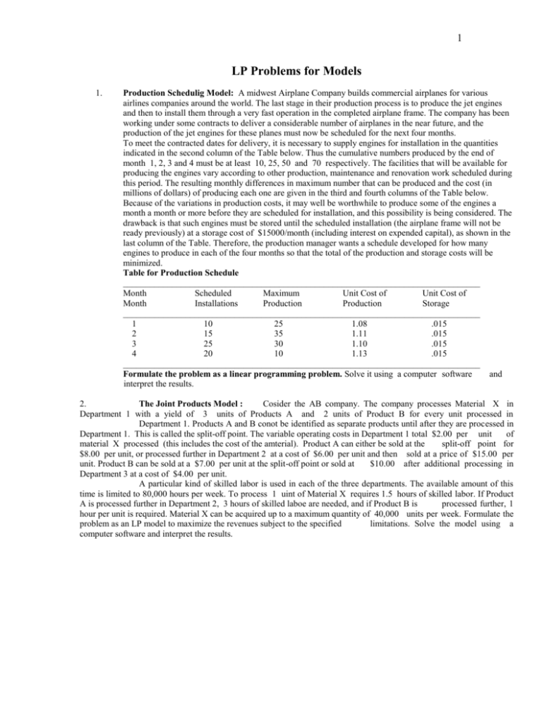
1
LP Problems for Models
1.
Production Schedulig Model: A midwest Airplane Company builds commercial airplanes for various
airlines companies around the world. The last stage in their production process is to produce the jet engines
and then to install them through a very fast operation in the completed airplane frame. The company has been
working under some contracts to deliver a considerable number of airplanes in the near future, and the
production of the jet engines for these planes must now be scheduled for the next four months.
To meet the contracted dates for delivery, it is necessary to supply engines for installation in the quantities
indicated in the second column of the Table below. Thus the cumulative numbers produced by the end of
month 1, 2, 3 and 4 must be at least 10, 25, 50 and 70 respectively. The facilities that will be available for
producing the engines vary according to other production, maintenance and renovation work scheduled during
this period. The resulting monthly differences in maximum number that can be produced and the cost (in
millions of dollars) of producing each one are given in the third and fourth columns of the Table below.
Because of the variations in production costs, it may well be worthwhile to produce some of the engines a
month a month or more before they are scheduled for installation, and this possibility is being considered. The
drawback is that such engines must be stored until the scheduled installation (the airplane frame will not be
ready previously) at a storage cost of $15000/month (including interest on expended capital), as shown in the
last column of the Table. Therefore, the production manager wants a schedule developed for how many
engines to produce in each of the four months so that the total of the production and storage costs will be
minimized.
Table for Production Schedule
________________________________________________________________________________
Month
Scheduled
Maximum
Unit Cost of
Unit Cost of
Month
Installations
Production
Production
Storage
________________________________________________________________________________
1
10
25
1.08
.015
2
15
35
1.11
.015
3
25
30
1.10
.015
4
20
10
1.13
.015
________________________________________________________________________________
Formulate the problem as a linear programming problem. Solve it using a computer software
and
interpret the results.
2.
The Joint Products Model :
Cosider the AB company. The company processes Material X in
Department 1 with a yield of 3 units of Products A and 2 units of Product B for every unit processed in
Department 1. Products A and B conot be identified as separate products until after they are processed in
Department 1. This is called the split-off point. The variable operating costs in Department 1 total $2.00 per unit
of
material X processed (this includes the cost of the amterial). Product A can either be sold at the
split-off point for
$8.00 per unit, or processed further in Department 2 at a cost of $6.00 per unit and then sold at a price of $15.00 per
unit. Product B can be sold at a $7.00 per unit at the split-off point or sold at
$10.00 after additional processing in
Department 3 at a cost of $4.00 per unit.
A particular kind of skilled labor is used in each of the three departments. The available amount of this
time is limited to 80,000 hours per week. To process 1 uint of Material X requires 1.5 hours of skilled labor. If Product
A is processed further in Department 2, 3 hours of skilled laboe are needed, and if Product B is
processed further, 1
hour per unit is required. Material X can be acquired up to a maximum quantity of 40,000 units per week. Formulate the
problem as an LP model to maximize the revenues subject to the specified
limitations. Solve the model using a
computer software and interpret the results.
2
3.
Gasoline Blending Model: One of the oil companies named as GOC. The GOC produces regular, premium
and low-lead gasoline by blending three constituents type 1, 2, and 3. The three constituents are available in limited
quantities and costs as follows:
constituent
Maximum Available / Day
Cost / Barrel
(Barrels)________________________________________
Type 1
2,000
$10.00
Type 2
3,000
7.50
Type 3
1,000
5.00
__________________________________________________________________________________________
The selling prices are $0.20 per gallon (there are 50 gallons in a barrel) for regular,
$0.30 for premium, and $0.15 for low-lead gasoline. The low-lead market is limited to 5,000 gallons per day.
The gasoline must be produced according to the following specifications.
Regular:
1. Not less than 20% of constituent of Type 1.
2. Not more than 30% of constituent of Type 3.
Premium:
1. Not less than 40% of constituent of Type 1.
2. Not less than 10% and not more than 20% of constituent of Type 2.
3. Not more than 10% of constituent of Type 3.
Low-Lead:
1. Not less than 30% of constituent of Type 2.
Formulate the problem as a Linear Programming problem so as to determine the volume of each gasoline to
sell that will maximize profits. Solve the model using a computer software and interpret the results.
4.
Coffee Blending Model: A coffee manufacturer blends four component coffee beans into three final blends of
coffee. The Table below summarizes the very precise recipes for the final coffee blends, the cost and
availability information for the four components, and the wholesale price per pound of the final blends. The
percentages in the body of the table indicate the percentage of each component to be used in each blend.
Table: Percentage of each component to be used in each blend
_______________________________________________________________________________________
Cost Per
Maximum Availability
Component
1
2
3
Pound
Each Week (Pound)
_____________________________________________________________________________________
1
20
35
10
$0.60
40,000
2
40
15
35
$0.80
25,000
3
15
20
40
$0.55
20,000
4
25
30
15
$0.70
45,000
_______________________________________________________________________________________
Wholesale Price/lb.
$1.25
$1.50
$1.40
_______________________________________________________________________________________
Weekly capacity for the processor's plant is 100,000 pounds, and the company wishes to operate at capacity.
There is no problem in selling the final blends, although there is a requirement that minimum production level of 10,000,
25,000 and 30,000 pounds, respectively, be met for blends 1, 2 and 3. The manufacturer wishes to determine the number
of pounds of each component which should be used in each blend so as to maximize total weekly profit.
Formulate the problem as an L.P. model. Solve the model using a computer software and interpret the
results.
5.
Multi-period Investment Problem. The Winnipeg Company has $200,000 available for
investment in a series of opportunities. There is no limit on the amount that can be invested in any
opportunity. Opportunity A is available in each of the next five years and can be repeated as many
times as desired. Foe every dollar invested in A at the beginning of a year, $1.20 will be returned two
years later. Similarly, opportunity B is available in each of the 5 years and, after 3 years, will return
$1.30 for every dollar invested at the beginning of a year. The other opportunities are available only
once. Opportunity C will return, at the beginning of the fifth year, $1.40 per dollar invested. But
opportunity C is available only at the beginning of the first year. Opportunity D, available at the
beginning of the second year will return $1.70 at the end of the fifth year per dollar invested.
3
Opportunity E is available at the beginning of the fourth year and will, in one year, return $1.40 per
dollar invested.
The company wishes to determine an investment scheme that allows the $200,000 to grow
by the greatest amount during the 5year period. Any realized gains on the $200,000 can also be
invested. Formulate a linear programming model that will fulfill company's wishes. Solve it using a
computer software and interpret the results.
6.
7.
Caterer's Problem. Suppose a caterer must supply clean napkins in the amounts 1,000; 700; 800; 1,200 and
1,500 for the next five days, respectively. The caterer has three alternatives for supplying napkins on any given
day:
(i)
Purchase new napkins at a cost of $1.00 each.
(ii) Utilize previously soiled napkins which have been cleaned by 1day (next day) service at a cost of $0.20
each.
(iii) Utilize previously soiled napkins which have been cleaned by a 2day service at a cost of $0.10 each.
Formulate an LP model for minimizing the total cost of supply. Solve the model using a computer
software and interpret the results.
City 1 produces 500 tons of waste per day, and city 2 produces 400 tons of waste per day. Waste must be
incinerated at incinerator 1 or incinerator 2, and each incinerator can process up to 500 tons of waste per day.
The cost to incinerate waste is $40/ton at incinerator 1 and $30/ton at incinerator 2. Incineration reduces each
ton of waste to 0.2 tons of debris, which must be dumped at one of two landfills. Each landfill can receive at
most 200 tons of debris per day. It costs $3 per mile to transport a ton of material (either debris or waste).
Distances (in miles) between locations are shown in Table below. Formulate an LP that can be used to
minimize the total cost of disposing off the waste of both cities.
TABLE
________________________________________________________________________
INCIN. 1
INCIN. 2
________________________________________________________________________
City 1
30
5
City 2
36
42
________________________________________________________________________
LANDFILL 1
LANDFILL 2
_____________
Incin. 1
5
8
Incin. 2
9
6
________________________________________________________________________
8.
A post office requires different numbers of full-time employees on different days of the week. The number of
full-time employees required on each day is given in the table below.
Table : Number of Employees Requirements
___________________________________________________________________________
Day 1(Mon) Day 2(Tue) Day 3(Wed) Day 4(Thu) Day 5(Fri) Day 6(Sat) Day 7(Sun)
17
13
15
19
14
16
11
___________________________________________________________________________
4
Union rules state that each full time employee must work five consecutive days and then receive two days off.
For example, an employee who works Monday through Friday must be off on Saturday and Sunday. The post
office wants to meet its daily requirements using only full-time employees. Formulate an LP model of the
problem that the post office can use to minimize the number of full-time employees that must be hired. Solve the
model using a computer software and interpret the results.
9
Hospital Administration: A local hospital administration is attempting to determine a work schedule for
registered nurses (R.N.'s). The union contract specifies that nurses are to work a normal day of six hours. Nurses
may work an additional three hours on an overtime work basis (at one and one half their hourly pay rate).
R.N.'s are paid on an average of $12 per hour. The administrator has determined a daily work schedule in which
the day is divided into eight three-hour shifts. The table below indicates the estimated demand for nurses per shift.
Period
____________________________________________________________________________________
1
2
3
4
5
6
7
8
Shift
12369123693 A.M.
6 A.M.
9 A.M.
12 Noon
3 P.M.
6 P.M.
9 P.M.
12 Midnight
Estimated
number of
required
R.N.'s 30
20
50
60
70
60
50
40
_____________________________________________________________________________________
Nurses are to start work at the beginning of one of these shifts and end work at the end of the following shift:
that is, unless they receive overtime. The contract specifies that (i) any nurses requested to work overtime will
receive full payment for three hours of overtime, even if they work less than three hours. Thus, the administrator
concludes that overtime, when assigned, should be for the maximum of three hours. The contract also specifies
that, on the average, at least 10 % of all nurses can expect overtime assignments. Let x t be the number of nurses
reporting to work at the beginning of period t who do not get overtime work and yt equal the number of nurses
reporting to work in period t who do work overtime. Formulate the problem as an LP model which will allow the
administrator to determine an assignment schedule which meets the shift requirements and contract specifications
at a minimum cost. Solve the model using a computer software and interpret the results.
10.
B.C. Wood Corporation (BSC) produces a special-purpose wood used in the housing and construction
industries. The sales department of BSC has received orders of 2400, 2200, 2700, and 2500 tons of wood
for each of the next 4 months. BSC can meet these demands by producing the wood, by drawing from its
inventory, or by using any combination of the two alternatives. The production costs per ton of wood during
each of the next four months are projected to be $7400, $7500, $7600, and $7650. Because costs are rising
each month, due to inflationary pressures, BSC might be better off producing more wood than it needs in a
given month and storing the excess. Production capacity, though, cannot exceed 4000 tons in any one
month. The monthly production is finished at the end of the month at which time the demand is met. Any
remaining wood is then stored in inventory at a cost of #120 per ton for each month that it remains there.
These data are summarized in the table below.
Table: Data for Production Planning Problem of BSC
____________________________________________________________________
Month
1
2
3
4
___________________________________________________________________________
Demand (Tons)
2400
2200
2700
2500
Production Cost ($/ton) 7400
7500
7600
7650
Inv. Cost($/ton/month)
120
120
120
120
___________________________________________________________________________
5
If the production level is increased from one month to the next, then the company incurs a cost of $50 per
ton of increased production to cover the additional labor and/or overtime. Each ton of decreased production
incurs a cost of $30 to cover the benefits of unused employees. The production during the previous month
was 1800 tons, and the beginning inventory is 1000 tons. Inventory at the end of the fourth month must be
at least 1550 to cover anticipated demand. Using linear programming formulate a production plan for BSC
that minimizes the total costs over the next four months.
11.
Tata Enterprises of India exports wood to customers in Eastern Europe, Canada and United States. Although
demand varies from quarter to quarter, contracts specify in advance the exact quarterly requirements. By
processing these contracts through the company's management information system (MIS), sales staff have
determined that Tata must deliver 2.5, 4, 3, and 4.5 million tons of wood in the next four quarters. There
are several ways to meet the requirements. One possibility is to "track" demand with production. Although
this option enables Tata to carry no inventory, it creates employee turnover and training problems
and
leaves substantial unused capacity at times. Another approach is to produce wood at a constant rate and
allow inventory to absorb the fluctuation in demand. Such an approach offers manufacturing efficiency, but it
typically involves a large inventory investment. Between these two extremes is the moderate option of
carrying some inventory while varying the production level somewhat.
Past experience indicates that the moderate option works best in Tata's operations. Management now must
determine the production and inventory levels that will minimize the costs of fulfilling the company's wood
contracts. Currently, Tata has 500,000 tons of wood in stock, and the company is manufacturing wood at the
rate of 3 million tons per quarter. By processing historical manufacturing data through the MIS, the
operations manager has forecasted that production costs will be $100, $120, $90, and $ 110 per ton
over the next four quarters. A similar MIS analysis of historical changeover (labor and facility adjustment)
data has indicated that it will cost $12 per ton to increase and $3 per ton to decrease production
from
one quarter to the next.
By processing historical purchasing, book keeping, and storage transactions through the MIS, the
operations manager also has estimated that it will cost 5% of the unit production cost in a quarter to
inventory wood for the corresponding quarter. Company accounting policy requires the operations manager
to asses his cost on the end-of-quarter inventory. At the end of four quarters, Tata wants no more than
400,000 tons and no less than 100,000 tons in stock. Using linear programming formulate a production plan
for Tata that minimizes the total costs over the next four periods.
6
1.
Given
(i)
Planning Horizon : 4 Months
(ii)
The following Table for Production Schedule
_______________________________________________________________
Unit Cost of Unit Cost of
Scheduled
Maximum
Production
Storage
Month
Installation
Production
(million $)
(million $)
_______________________________________________________________
1
10
25
1.08
.015
2
15
35
1.11
.015
3
25
30
1.10
.015
4
20
10
1.13
.015
________________________________________________________________
Decision Variables. Let
xij = # of engines produced in month i for installation in month j, (i < j)
(Therefore, for i > j, xij = 0)
cij = unit production and storage cost associatedwith each unit of xij, (i < j)
Thus we have the cost matrix Cij as follows.
Month Produced
1
2
3
Month Installed
2
3
4
1
1.080 1.095 1.110 1.125
1.110 1.125 1,140
1.100 1.115
4
-
-
-
1.130
Max. Prodn.
25
35
30
10
The production matrix Xij is
Month Produced
Month Installed
2
3
4
1
Max. Prodn.
1
2
x11
-
x12
x22
x13
x23
x14
x24
25
35
3
4
-
-
x33
-
x34
x44
30
10
7
Then the model is
4
O.F.
Min. z =
4
 c x
i 1 j 1
ij ij
where i < j,
Constraints.
1.
Maximum Production Constraints
x11 + x12 + x13 + x14
x22 + x23 + x24
x33 + x34
x44
2.
(iii)
Installation Constraints
x11
x12 + x22
x13 + x23 + x33
x14 + x24+ x34 + x44
Nonnegativity Constraint:
≤ 25
≤ 35
≤ 30
≤ 10
= 10
= 15
= 25
= 20
xij ≥ 0 for i = 1, 2, 3, 4, j = 1, 2, 3, 4.
NOTE. In above definitions if we assume
xij = # of engines produced in month i for installation in month j for all i and j,
we then take
cij = unit production and storage cost associatedwith each unit of xij,
where,
unit production and storage cost associatedwith each unit of xij, (i < j)
cij =
M,
a very large number if i > j .
Then the model is
4
Min. z =
4
 c x
i 1 j 1
ij ij
Constraints.
1.
Maximum Production Constraints
x11 + x12 + x13 + x14 ≤
x21 + x22 + x23 + x24 ≤
x31 + x32 + x33 + x34 ≤
x41 + x42 + x43 + x44 ≤
25
35
30
10
8
2.
Installation Constraints
x11 + x21 + x31 + x41 = 10
x12 + x22+ x32 + x42 = 15
x13 + x23 + x33 + x43 = 25
x14 + x24+ x34 + x44 = 20
3. Nonnegativity Constraint: xij ≥ 0 for i = 1, 2, 3, 4, j = 1, 2, 3, 4.
2.
Let
xA1 = quantity of Product A sold at the split-off point.
xA2 = quantity of Product A sold after processing in Dept. 2
xB1 = quantity of Product B sold at the split-off point.
xB2 = quantity of Product A sold after processing in Dept. 3
xq = quantity of Product X used in Dept. 1
pA1 = unit net revenue of Product A sold at the split-off point. = $8.00
pA2 = unit net revenue of Product A sold after processing in Dept. 2 = $15  $6 =9
pB1 = unit net revenue of Product B sold at the split-off point. = $7.00
pB2 = unit net revenue of Product B sold after processing in Dept. 3 = $10  $4 =6
cq = unit cost Product X used in Dept. 1 = $2.00
Sell A @
$8.00, xA1
A = 3 xq
Dept. 2, xA2
Cost = $6.00
Labor = 3 Hrs./unit
X = xq
Sell @
$15.00
xA2
Dept.1
cq = $2
Labor = 1.5 Hrs./unit
Sell B @
$7.00, xB1
B = 2 xq
Dept. 2, xB2
Cost = $6.00
Labor = 3 Hrs./unit
Sell @
$10.00
xB2
9
Objective Function: Maximize the total net revenue z.
Maximize z = 8 xA1 + 9 xA2 + 7 xB1 + 6 xB2  2 xq
Constraints.
1. Weekly Consumption of xq ,
2. Skilled Labor Consumption.
3 xA2 + 1 xB2
xq ≤ 40,000
+ 1.5 xq ≤ 80,000
3. Each unit of xq produces 3 units of A and 2 units of B.
xA1 + xA2 = 3 xq
xB1 + xB2 = 2 xq
4. Nonnegativity.
xA1 , xA2 , xB1 , xB2 , xq ≥ 0
3. We define the Decision Variables as follows. Let
j = Regular (R), Premium (P), and Low-Lead (L)
Gj = Total Gasoline of Type j j = R, P, L
Ci = Total Constituent of Type i i = 1, 2, 3
xij = Amount (in Barrels) of Constituent of type i in gasoline of type j, i = 1, 2, 3;
j = R, P, L.
Gasoline Type
Const. Type R
P
L
1
2
3
S.P. of Gasoline/ gallon
S.P. of Gasoline/ Barrel
x1R
x2R
x3R
x1P
x2P
x3P
$.20
$.30
$10.00 $15.00 $7.50
GR
Therefore,
GR = x1R + x2R + x3R
GP = x1P + x2P + x3P
GL = x1L + x2L + x3L
GP
x1L
x2L
x3L
C1
C2
C3
$.15
GL
C1 = x1R + x1P + x1L
C2 = x2R + x2P + x2L
C3 = x3R + x3P + x3L
10
Profit, z = Revenue  Cost
Objective Function:
Max. z = (10 GR + 15 GP + 7.5 GL)  [10 C1 + 7.5 C2 + 5 C3]
= 2.5 x2R + 5 x3R+ 5 x1P + 7.5 x2P + 10x3P  2.5 x1L + 2.5 x3L
Constraints.
1.
Constituent Availability Constraints.
Type 1:
x1R + x1P + x1L ≤ 2,000
Type 2:
x1R + x2P + x2L ≤ 3,000
Type 3:
x3R + x3P + x3L ≤ 1,000
2.
Market Potential for Low-Lead Gasoline Constraint.
x1L + x2L + x3L ≤ 100
(5,000 gallons)
3.
Technological (Specification) Constraints.
Regular:
Amount of Constituent 1 in Regular Gasoline
_____________________________________ ≥ .20
Total Amount of Regular Gasoline
(i)
x1R
x1R  x 2R  x3 R ≥ .20

i.e.
.8 x1R + .2 x2R + .2 x3R ≤ 0
Similarly,
(ii)
Amount of Constituent 3 in Regular Gasoline
_____________________________________ ≤ .30
Total Amount of Regular Gasoline
.3 x1R .3 x2R + .7 x3R ≤ 0
Premium.
(i)
(ii)
and
(iii)
.6 x1P + .4 x2P + .4 x3P ≤ 0
.1 x1P  .9 x2P + .1 x3P ≤ 0,
.2 x1P  .8 x2P  .2 x3P ≤ 0
.1 x1P  .1 x2P + .9 x3P ≤ 0
Low- Lead.
. 3 x1L  .7 x2L + .3 x3L ≤ 0,
11
4.
4.
Nonnegativity.
All
xij ≥ 0, for i = 1, 2, 3;
j = R, P, L.
We first define the Decision Variables. Let
xij = number of pounds of component i used in final blend j, i= 1, 2,3,4; j =1,2,3.
Therefore, we have
________________________________________________________________________
Final Blend number of pounds
Cost Per
Maximum Availability
Component
1
2
3
Pound
Each Week (Pound)
(pounds)
________________________________________________________________________
1
x11
x12
x13
$0.60
40,000
2
x21
x22
x23
$0.80
25,000
3
x31
x32
x33
$0.55
20,000
4
x41
x42
x43
$0.70
45,000
________________________________________________________________________
Wholesale Price/lb. $1.25 $1.50 $1.40
________________________________________________________________________
Objective Function. To maximize weekly profit z , say. Therefore, we have
4
4
4


$ 1.25 xi1  1.50 xi 1  1.40  xi1



i1
i 1
Max. z =  i 1
4
4
4
 4

 $ .60 x1 j .8 x 2 j .55 x 3j .7 x4 j


 i1

i 1
i 1
i1
= .65 x11 + .9x12 + .8 x13 + .45 x21 + .7 x22 + .6 x23
+ .7 x31 + .95 x32 + ..85 x33 +.55 x41 +.8 x42 + ..8 x43
Constraints.
1.
Final Blend of Type 1.
Amount of Component 1 in Blend of Type 1
_____________________________________ = .20
Total Amount ofBlend of Type 1
(i)

i.e.

x11
x11  x21  x 31  x41 = .20
.8 x11 + .2 x21 + .2 x31 + .2 x41 = 0
12
Similarly
(ii)
(iii)
(iv)
2.
.4 x11  .6x21 + .4x31 + .4x41 = 0
.15 x11 + .15 x21  .85 x31 + .15 x41 = 0
.25 x11 + .25 x21 + .25 x31  .75 x41 = 0
Final Blend of Type 2.
.65 x12 + .35 x22 + .35 x32 + .35 x42 = 0
.15 x12  .85 x22 + .15 x32 + .15 x42 = 0
.20 x12 + .20 x22  .80 x32 + .20 x42 = 0
.30 x12 + .30 x22 + .30 x32  .70 x42 = 0
3.
Final Blend of Type 3.
.90 x13 + .10 x23 + .10 x33 + .10 x43 = 0
.35 x13  .65 x23 + .35 x33 + .35 x43 = 0
.40 x13 + .40 x23  .60 x33 + .40 x43 = 0
.15 x13 + .15 x23 + .15 x33  .85 x43 = 0
4.
Plant Capacity.
(x11 + x12 + x13) + (x21 + x22 + x23) + (x31 + x32 + x33) + (x41 + x42 + x43) = 100,000
5.
Component Availabilities.
x11 + x12 + x13 ≤ 40,000
x21 + x22 + x23 ≤ 25,000
x31 + x32 + x33 ≤ 20,000
x41 + x42 + x43 ≤ 45,000
6.
Minimum Production Level Requirements.
x11 + x21 + x31 + x41 ≥ 10,000
x12 + x22 + x32 + x42 ≥ 25,000
x13 + x23 + x33 + x43 ≥ 30,000
Nonnegativity.
All xij ≥ 0 for 1 = 1, 2, 3, 4;
5.
Let
j = 1, 2, 3.
13
Aj = $ invested in opportunity A available at the beginning of year j, j = 1, 2, 3, 4
Bj = $ invested in opportunity B available at the beginning of year j,
Cj = $ invested in opportunity C available at the beginning of year j,
Dj = $ invested in opportunity D available at the beginning of year j,
Ej = $ invested in opportunity E available at the beginning of year j,
Let Sj represent funds that remain idle in j-th year, j = 1, 2, . . . , 5.
$200,000
Available
j = 1, 2, 3
j = 1 only
j = 2 only
j = 4 only
1
2
3
4
5
_________________________________________________________
. . . . . A1 . . . . . . . . . .  $1.20 A1
. . . . . B1 . . . . . . . . . . . . . . . . . . . . $1.30 B1














. . . . . C1 . . . . . . . . . . . . . . . . . . . . . . . . . . . . . . . $1.40 C1
. . . . . S1 . $1 S1
. . . . . A2 . . . . . . . . . . . $1.20 A2
. . . . . B2 . . . . . . . . . . . . . . . . . . . . . . $1.30 B2
. . . . . D2 . . . . . . . . . . . . . . . . . . . . . . . . . . . . . . . . $1.70 D2

 . . . . . S2 . .$1 S2



. . . . . A3 . . . . . . . . . . . . .$1.20 A3
. . . . . B3 . . . . . . . . . . . . . . . . . . . . . . . $1.30 B3



. . . . . S3 . . .$1 S3




. . . . . A4 . . . . . . . . . . . . . $1.20 A4





. . . . . E4 . . . $1.40 E4





. . . . . S4 . . . $1S4 







. . . . . S5 . . .$1 S5
__________________________________________________________
Objective Function. It is written in terms of those variables that generate money at the end of
Fifth year, and the returns from all other opportunities at the end of other years appear in the
constraints.
Therefore, we have,
Max z = 1.70 D2 + 1.3 0 B3 + 1.20 A4 + 1 S5
Constraints. We must ensure that the investment in each year does not exceed the total money
available.
14
Year 1: A1 + B1 + C1 + S1 = 200,000
Year 2: A2 + B2 + D2 + S2 = S1
Year 3:
A3 + B3 + S3 = S2 + 1.20 A1
Year 4:
A4 + E4 + S4 = S3 + 1.30 B1 + 1.20 A2
Year 5:
S5 = S4 + 1.40 C1 + 1.30 B2 + 1.20 A3 + 1.40 E4
Nonnegativity. Aj ≥ 0, j = 1, 2, 3, 4; Bj ≥ 0, j = 1, 2, 3; C1 ≥ 0, D2 ≥ 0, E4 ≥ 0,
Sj ≥ 0, j = 1, 2, 3, 4, 5.
6.
Let
xj = # of New napkins purchased on Day j , j = 1, 2, 3, 4, 5
yj = # of napkins sent for cleaning to one day service on Day j , j = 1, 2, 3, 4
zj = # of napkins sent for cleaning to two day service on Day j , j = 1, 2, 3
Objective Function :
Min. z = $1 (x1 + x2 + x3 + x4 + x5) + $0.2 (y1 + y2 + y3 + y4)
+ $0.1 (z1 + z2 + z3)
Constraints:
(Day 1)
(Day 2)
x1
= 1000
x2
(Day 3)
+ y1
x3
(Day 4)
= 700
+ y2
+ z1
x4
(Day 5)
= 800
+ y3
x5
+ y4
+ z2
= 1200
+ z3 = 1500
Constraints for Soiled Napkin
(Day 1)
y1
+ z1
(Day 2)
y2

(y1 + y2) + (z1 + z2)
≤ 1700
(Day 3)
(y1+y2+y3) + (z1+z2+z3)
≤ 2500
(Day 4)
(y1+y2+y3+y4) + (z1 + z2+ z3)
+ z2
≤ 1000
≤ 700+[1000  (y1+ z1)]
≤ 3700
15
(Day 5)
(y1+y2+y3+y4)+(z1+z2+z3)
≤ 5200
Nonnegativity: xj ≥ 0, yj ≥ 0, zj ≥ 0,
j = 1, 2, 3, 4, 5
16
7.
DECISION VARIABLES:
xij = Amount of waste shipped from city i to Incin. j,
j = 1, 2
yjk = Amount of waste shipped from city i to Incin. j, j, k = 1, 2
Then,
Constraints:
City 1 x11 + x12 = 500
Incin. 1
x11 + x21 ≤ 500
City 2: x21 + x22 = 400
Incin. 2:
x12 + x22 ≤ 400
City and Incinerator
.2 (x11 + x21) = y11 + y12 , .2 (x12 + x22) = y21 + y22
Landfill:
y11 + y12 ≤ 200,
y21 + y22 ≤ 200
Total Cost:
z = Total Cost of Transportation + Total Cost of Incineration
17
= [90 x11 + 15 x12 + 108 x21 + 126 x22 + 15y11 + 24 y12
27 y21 + 18 y22] + [40 (x11 + x21) + 30 (x12 + x22)]
8.
Let , for t = 1, 2, . . . . , 7
xt = # of employees reporting to work at the begining of Day t, t = 1, 2, . . , 7
then, the total number of Employees = x1 + x2 + x3 + x4 + x5 + x6 + x7
Objective Function: Min. z = x1 +x2 +x3 +x4 +x5 +x6 +x7
Constraints.
Shift 1:
x1 + x7 + x6 + x5 + x4 ≥ 17
Shift 2:
x2 + x1 + x7 + x6 + x5 ≥ 13
Shift 3:
x3 + x2 + x1 + x7 + x6 ≥ 15
Shift 4:
x4 + x3 + x2 + x1 + x7 ≥ 19
Shift 5:
x5 + x4 + x3 + x2 + x1 ≥ 14
Shift 6:
x6 + x5+ x4 + x3 + x2 ≥ 16
Shift 7:
x7 + x6 + x5 + x4 + x3 ≥ 11
Nonnegativity Constraint. All xt ≥ 0, t = 1, 2, . . , 7
9.
Let , for t = 1, 2, . . . . , 8
xt = # of nurses reporting to work at the begining of period t , and who do not
get overtime
yt = # of nurses reporting to work at the begining of period t , and who do get
overtime
8
8
 72x  126y
t
t
i1
then, the cost of wages paid to all nurses = i 1
Objective Function: Min. z = 72 (x1 +x2 +x3 +x4 +x5 +x6 +x7+x8)
+ 126 (y1 +y2 +y3 +y4 +y5 +y6+y7+y8)
No. of Nurses on duty during shift t = xt +yt +xt-1 +yt-1 +yt-2
No. of Nurses on duty during shift t
Constraints.
Shift 1:
x1 + y1 + x8 + y8 + y7
Shift 2:
x2 + y2 + x1 + y1 + y8
Shift 3:
x3 + y3 + x2 + y2 + y1
Shift 4:
x4 + y4 + x3 + y3 + y2
Shift 5:
x5 + y5 + x4 + y4 + y3
Shift 6:
x6 + y6 + x5 + y5 + y4
Shift 7:
x7 + y7 + x6 + y6 + y5
= xt +yt +xt-1 +yt-1 +yt-2
≥
≥
≥
≥
≥
≥
≥
30
20
50
60
70
60
50
18
Shift 8:
x8 + y8 + x7 + y7 + y6 ≥ 40
Contract:
y1 +y2 +y3 +y4 +y5 +y6+y7+y8 ≥ .10 [(x1 +x2 +x3 +x4 +x5 +x6
+x7+x8) + (y1 +y2 +y3 +y4 +y5 +y6+y7+y8)]
Nonnegativity Constraint. All
10.
xt, yt ≥ 0, t = 1, 2, . . , 8
are nonnegative.
Formulation.
Decision Variables are defined as follows: Let
x = the number of tons of wood to produce during month 1
1
x = the number of tons of wood to produce during month 2
2
x = the number of tons of wood to produce during month 3
3
x = the number of tons of wood to produce during month 4
4
I = Inventory in tons of wood at the beginning of month 1
1
I = Inventory in tons of wood at the beginning of month 2
2
I = Inventory in tons of wood at the beginning of month 3
3
I = Inventory in tons of wood at the beginning of month 4
4
S = the number of tons of increased production in month 1
1
D = the number of tons of decreased production in month 1
1
S = the number of tons of increased production in month 2
2
D = the number of tons of decreased production in month 2
2
S = the number of tons of increased production in month 3
3
D = the number of tons of decreased production in month 3
3
S = the number of tons of increased production in month 4
4
D = the number of tons of decreased production in month 4
4
Objective.
To minimize the overall total cost. Let the overall cost be denoted by z.
Then,
z = total production cost + total inventory cost + total cost due to change in production
Now,
total cost due to change in production
4
=
•
cost due to increase in month i + cost due to decrease in month i
i=1
4
=
•
50 Si + 30 Di
i=1
Therefore, we have
Minimize z = (7400 x + 7500 x + 7600 x + 7650 x ) + (120 I + 120 I + 120 I + 120 I )
1
2
3
4
1
2
3
4
(50 S + 50 S + 50 S + 50 S ) + (30 D + 30 D + 30 D + 30 D )
1
2
3
4
1
2
3
4
Constraints.
1.
Boundary Conditions
Initial and Final Inventory Constraints.
(Initial Inventory)
I1 = 1000
19
2.
3.
4.
(Ending Inventory)
I5 ≥ 1500
Production Capacity Constraints.
x ≤ 4000,
x ≤ 4000,
1
2
x ≤ 4000,
3
Inventory Balance Constraints.
I +
(month 1)
1
I
+
(month 2)
2
I +
(month 3)
3
I +
(month 4)
4
I
I
I
I
2
3
4
5
= 2400
= 2200
= 2700
= 2500
Change in Production Constraints. Let
x = production during the previous month
0
= 1800
(given in the problem)
(month 1)
(month 2)
(month 3)
(month 4)
5.
x 
1
x 
2
x 
3
x 
4
x ≤ 4000
4
x  x
1
0
x  x
2
1
x  x
3
2
x  x
4
3
+ D 
1
+ D 
2
+ D 
3
+ D 
4
S
1
S
2
S
3
S
4
= 0
= 0
= 0
= 0
Nonegativity Constraints. All variables are nonnegative.
Solution. x = 1800, x = 1800, x = 2700, x = 4000; I = 1000, I = 400, I = 0, I = 0, I = 1500,
1
2
3
4
1
2
3
4
5
S = 0, S = 0, S = 900, S = 1300; D = 0, D = 0, D = 0, D = 0, OFV = 78,218,000.
1
2
3
4
1
2
3
4
The optimal production plan can be summarized as follows.
Month
_______________________________________________________
1
2
3
4
________________________________________________________________________________
Beginning Inventory
1000
400
0
0
Amount Produced
1800
1800
2700
4000
Ending Inventory
400
0
0
1500
_________________________________________________________________________________
11.
Decision Variables are defined as follows: Let
x1 = the number of tons of wood to produce during period 1
x2 = the number of tons of wood to produce during period 2
x3 = the number of tons of wood to produce during period 3
x4 = the number of tons of wood to produce during period 4
I1 = Inventory in tons of wood at the beginning of period 1
I2 = Inventory in tons of wood at the beginning of period 2
20
I3 = Inventory in tons of wood at the beginning of period 3
I4 = Inventory in tons of wood at the beginning of period 4
21
S1
D1
S2
D2
S3
D3
S4
D4
=
=
=
=
=
=
=
=
the number of tons of increased production in period 1
the number of tons of decreased production in period 1
the number of tons of increased production in period 2
the number of tons of decreased production in period 2
the number of tons of increased production in period 3
the number of tons of decreased production in period 3
the number of tons of increased production in period 4
the number of tons of decreased production in period 4
Objective. To minimize the overall total cost. Let the overall cost be denoted by z.
Then,
z = total production cost + total inventory cost + total cost due to change in
production
Now,
total cost due to change in production
4
=
•
cost due to increase in period i + cost due to increase in period i
i=1
4
=
•
12 Si + 3 Di
i=1
Therefore, we have
Maximize z = (100 x1 + 120 x2 + 90 x3 + 110 x4) + (5 I1 + 6 I2 + 4.5 I3 + 5.5 I4)
(12 S1 + 12 S2 + 12 S3 + 2 S4) + (3 D1 + 3 D2 + 3 D3 + 3 D4)
Constraints.
1.
Boundary Conditions.
Initial and Final Inventory Constraints.
2.
4.
(Initial Inventory)
I1 = 500,000
(Ending Inventory)
I5 ≤
400,000,
I5 ≥ 100,000
Inventory Balance Constraints.
I1 + x1  I2 = 2,500,000
(quarter 1)
I2 + x2  I3 = 4,000,000
(quarter 1)
(quarter 1)
I3 + x3  I4 = 3,000,000
(quarter 1)
I4 + x4 I5 = 4,500,000
Change in Production Constraints.
Therefore,
Let
x0 = production during the previous period
x0 = 3,000,000
22
(quarter 1)
(quarter 2)
(quarter 3)
(quarter 4)
5.
Nonegativity Constraints.
x  x
1
0
x  x
2
1
x  x
3
2
x  x
4
3
+ D 
1
+ D 
2
+ D 
3
+ D 
4
S
1
S
2
S
3
S
4
= 0
= 0
= 0
= 0
All variables are nonnegative.
23
7.
DECISION VARIABLES:
xij = Amount of waste shipped from city i to Incin. j,
i, j = 1, 2
yjk = Amount of waste shipped from city i to Incin. j, j, k = 1, 2
Constraints:
City 1 x11 + x12 = 500
City 2: x21 + x22 = 400
Incin. 1
Incin. 2:
x11 + x21 ≤ 500
City and Incinerator
x12 + x22 ≤ 400
.2 (x11 + x21) = y11 + y12 ,
.2 (x12 + x22) = y21 + y22
Landfill 1. y11 + y21 ≤ 200,
Landfill 2. y12 + y22 ≤ 200
Nonnegative : al variables >= 0
24
Total Cost: z = Total Cost of Transportation + Total Cost of Incineration
= [90 x11 + 15 x12 + 108 x21 + 126 x22 + 15y11 + 24 y12 +27 y21 + 18 y22]
+ [40 (x11 + x21) + 30 (x12 + x22)]