Chapter 3
Shape-Adaptive Image Compression
Algorithm
The JPEG image compression standard can achieve great compression ratio,
however, it does not take advantage of the local characteristics of the given image
effectively. Therefore, the new image compression algorithm called shape-adaptive
image compression algorithm, abbreviated SAIC, was proposed. Instead of segmenting
the whole image into several square blocks and applying transform coding, quantization,
and entropy coding to each block, the SAIC algorithm segments the whole image into
several image segments, and each image segments has its own local characteristics.
Because of the high correlation of the luma and chroma in each image segment, the
SAIC can achieve higher compression ratio and better image quality than the
conventional block-based image compression algorithm such as JPEG.
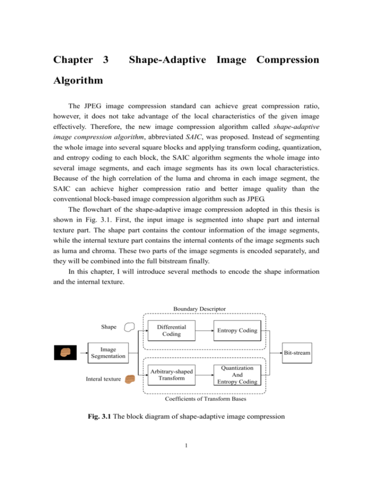
The flowchart of the shape-adaptive image compression adopted in this thesis is
shown in Fig. 3.1. First, the input image is segmented into shape part and internal
texture part. The shape part contains the contour information of the image segments,
while the internal texture part contains the internal contents of the image segments such
as luma and chroma. These two parts of the image segments is encoded separately, and
they will be combined into the full bitstream finally.
In this chapter, I will introduce several methods to encode the shape information
and the internal texture.
Boundary Descriptor
Shape
Differential
Coding
Entropy Coding
Image
Segmentation
Interal texture
Bit-stream
Arbitrary-shaped
Transform
Quantization
And
Entropy Coding
Coefficients of Transform Bases
Fig. 3.1 The block diagram of shape-adaptive image compression
1
Image Compression Tutorial
3.1 Coding of Binary Shape Image
In shape-adaptive image compression, we must exploit some image segmentation
algorithms to capture the shape information of the source image. After the shape
information is obtained, we must use some shape compression methods to reduce the
quantity of data. In this thesis, I adopt the method introduced in and run length coding
to reduce the quantity of data.
3.1.1 Differential Coding of Binary Shape Image
As we know, high correlation often exists between the neighboring pixels in the
natural images. These high correlation characteristics still exist in the binary image, and
we can apply some methods to reduce the correlation. Because there are only 2 levels in
the binary shape image, it is not proper for us to use the common image compression
methods such as JPEG, JPEG 2000 and so on. One method to reduce the correlation is
the differential coding, which is introduced in section 3.1.2, and it is very efficient for
the binary shape image. After differential coding, the probability of white pixel will be
much less than that of the black pixel, so we can apply the coding algorithm in Error!
Reference source not found. or run length coding to achieve compression.
If we apply the differential coding directly, which is defined in (3.1), then the
symbol set may become {-1,0,1}. For example, if aij=0 and ai,j-1=1, then the value of dij
is -1.
 aij
dij  
aij  ai , j 1
j0
j  1, 2,..., M
(1.1)
where aij is the pixel value of (i,j)th element in the binary image, and the size of the
image is N×M
Therefore, the differential method in (1.1) cannot be applied to the binary shape
image directly. In Error! Reference source not found., the George et al. Proposed a
new differential algorithm with XOR(Exclusive-OR) for the binary image. The
differential coding method is defined in (3.2).
aij

dij  
 aij  ai , j 1  aij  ai , j 1
j0
j  1, 2,..., M
(1.2)
where  means Exclusive-OR.
We take the binary lena image for experiment. The original binary lena image and
2
Image Compression Tutorial
the binary difference image is shown in Fig. 3.1. It is worth noting that the differential
coding is applied along the horizontal direction and along the vertical direction
afterward. As can be seen from the simulation result, the probability of 1 is much less
than that of 0, which makes us easier to process and compress it.
(a) The original binary lena image
(b) The binary difference image
Fig. 3.2 The binary Lena image before and after differential coding
In the end of this section, I also perform some simulations on our binary shape
image, and the simulation results are shown in Fig 3.3.
(a) The binary shape image
(b) The binary difference image
Fig. 3.3 The binary shape image before and after differential coding
3.1.2 Block Coding of Sparse Binary Image
After differential coding, we can apply the probability characteristics to achieve
compression. As we know, the data will become geometric distribution after differential
coding. However, the symbol set contains 2 elements only, so the Golomb codes can not
be applied. In Error! Reference source not found., the coding method designed for the
sparse binary image (most elements in the binary image are 0) was proposed. The
method is called Block Coding method and the flow of this algorithm is as follows. One
3
Image Compression Tutorial
example is shown in Fig. 3.4.
Block Coding Algorithm
1.
Map the 2D image to 1D row-stacked form, and the number of elements must
be modeled as 2 M .
2.
3.
4.
5.

 np  
Define a  log 2 
  , where n is the total number of pixels in the binary
 ln 2  

image, and p is the probability of finding “1“.
Segment the 1D data string into 2 a blocks, and each block contains 2b bits.
Therefore, M=a+b.
We introduce a comma ‘0 ‘ to seperate the blocks.
There two conditions
5.1 If there is no 1 in one block, then no coding in needed for the block
5.2 If there are 1s in one block, then assign each 1 a prefix “1“ followed by b
bits to indicate its location in the block.
0
1
0
0
0
1
1
0
0
0
0
0
0
0
0
0
Step 1, 2
0100,
0110,
A 1 in location 1(012)
101
0000,
0000
Step 3
0 101110 0
A 1 in location 1(012)
0
A 1 in location 2(102)
Step 4
101010111000
Final Bitstream
4
Image Compression Tutorial
Fig. 3.4 One example of block coding
After differential coding the binary shape image, the probability of finding “1“ in
the difference image ( Fig. 3.3 (b) ) is 0.024 and the probability of finding “0“ is 0.976.
Therefore, we can exploit the block coding algorithm to compress the difference image.
The data quantity of the difference image after block coding is 228 bytes. If we encode
each image segemnt in the shape image separately, the quantity of data after block
coding is 154 bytes as shown in Fig. 3.5. As can seen from the simulation result, the
lower the probability of finding “1“, the higher the compression ratio.
Object
Diff img
Storage
35 bytes
2 bytes
54 bytes
13 bytes
33 bytes
19 bytes
CR
2.578755
40.00000
2.222222
3.676768
2.155894
2.395973
Prob(1)
0.0597
0.0025
0.0813
0.0385
0.0705
0.0672
Fig. 3.5 The data quantity and compression ratio of each element
Although this coding method cannot achieve high coding efficiency than that of the
Fourier descriptor, the contour of all image segments can be perfectly reconstructed
because this is a lossless compression algorithm.
3.2 Coding of Internal Texture
In block-based transform coding algorithms, the source image is segmented into
several small blocks with fixed NN size. In each block, all the pixel values are fully
defined, and the DCT can be used to encode these blocks efficiently. However, for the
image segments in shape-adaptive image compression, only a portion of pixel values is
defined. One straight method to solve this problem is to fill zero values outside the
contour and treat the filled contour block as a rectangular block. However, padding
zeros will introduce unnecessary high frequency components across the object boundary,
so the high-frequency transform coefficients increase and the compression performance
seriously degrade. We show one example of the padding method in Fig. 3.6.
5
Image Compression Tutorial
0
0
0
0
75 96
0
0
105 98 99 101 73 85 66 60
0 100 97 89 94 87 64 55
0
0
84 94 90 81 71 66
0
0
93 86 94 81 70
0
0
0
0
86 86 81 72
0
0
0
0
98 97 78
0
0
0
0
0 105 104 0
0
0
2D-DCT
395.1
 82.0

 -83.2

 -71.2
 -72.6

 -57.3
 -43.8

 -14.3
19.3
2.2
-4.7 -10.7 
-5.8 -68.3 -31.4 42.4 7.0 
44.6 52.3 -40.1 -10.9 -24.9 

-31.8 -8.7 76.8 -14.7 15.2 19.6 -1.1 
-28.0 -24.0 -2.8 15.1
5.1 21.9 37.1 

-50.6 -21.0 18.7
6.2 -31.4 19.4 -16.8 
-27.9 -9.4 6.5 -16.4 -21.6 -31.7 2.0 

13.5 -30.1 -2.0 -28.0 -27.5 6.4
3.8 
-57.5 -205.8 36.5
18.2
40.4
69.7
17.9
Fig. 3.6 Arbitrary DCT Transform by padding zeros outside the boundary
Instead of filling data outside the image boundary and applying rectangular
transform, we can focus on the defined image contents only, i.e. P(x, y) values within
region B. Mathematically, let’s define SR as the linear space spanned over the whole
square block R, SB as the subspace spanned over the irregular region B only. For
example, in Fig. 3.7 (a), space SR has a dimension equals to 9, while the dimension of
subspace SB equals to 6. One possible basis for subspace SB is shown in Fig. 3.7 (b).
Each basis matrix has a single non-zero element only.
SB Image Segment
0
0
0
0
1
0
0
0
0
1
0
0
0
0
0
0
1
0
0
0
0
0
0
0
0
0
0
0
0
1
0
0
0
0
0
0
0
0
0
0
0
1
0
0
0
0
0
0
0
0
0
0
0
1
SR
3х3 pixel
Fig. 3.7 (a) An irregular-shape image segment in a 33 block area
(b) A canonical basis of the subspace
Every arbitrary-shape image segment, P(x, y), can be considered as a vector in SB.
To represent this vector completely, we can find a set of independent vectors, say bi, in
SB and describe P(x, y) as a linear combination of bi’s. The distinction between this
approach and that in the previous section is that the whole problem domain now is
confined in the subspace SB only. We don’t have to worry about the redundant data
outside the image boundary, i.e. vector component outside subspace SB. If we still want
to use traditional block-based transform bases, say fi (e.g. DCT basis), we can project
6
Image Compression Tutorial
these basis functions into subspace SB,
fˆi  Project( fi , SB )
(1.3)
and describe vector P(x, y) as a linear combination of fˆi ’s. Actually, the above
projection is very simple. It just removes the components of fi outside subspace SB.
An important issue remains now is how to find optimal basis functions in subspace
SB such that we can use the least number of coefficients to reconstruct the image
segment vector with satisfactory errors. The above formulation does provide a very
flexible platform to derive new transform bases and evaluate their performance.
3.2.1 Arbitrary-Shape transform based on Gram-Schmidt Process
In this subsection, we introduce the proposed transform method to remove
correlation based on the Gram-Schmidt process. To compare with the 88 DCT, we use
the same image segment in Fig. 3.8 whose height and width are both eight, as shown in
Fig. 3.8 (a). Fig. 3.8 (b) is its binary shape image by filling with one’s in the position
inside the boundary of the shape and filling with zeroes otherwise.
0
0
0
0
75 96
0
0
0
0
0
0
1
1
0
0
105 98 99 101 73 85 66 60
1
1
1
1
1
1
1
1
0 100 97 89 94 87 64 55
0
1
1
1
1
1
1
1
0
0
84 94 90 81 71 66
0
0
1
1
1
1
1
1
0
0
93 86 94 81 70
0
0
0
1
1
1
1
1
0
0
0
0
86 86 81 72
0
0
0
0
1
1
1
1
0
0
0
0
98 97 78
0
0
0
0
0
1
1
1
0
0
0
0
0 105 104 0
0
0
0
0
0
1
1
0
0
0
Fig. 3.8 (a) An arbitrary-shape image segment f and (b) its shape matrix
Similar to the 88 DCT, we can get the HW bases of the image segment f. We
multiplying the original HW DCT basis by the shape matrix shown in Fig. 3.8 (b) and
the result is shown in Fig. 3.9. Because the point number M of is less than HW, we can
know that the HW bases are not orthogonal. Before we use the Gram-Schmidt process
to reduce the bases to M orthogonal ones, we reorder the HW bases by the zigzag
reordering matrix. The reason to reorder is that the low frequency components
7
Image Compression Tutorial
concentrate on the left-top position and is more important to the high frequency
components which concentrate on the right-bottom position. After zigzag scan
reordering, we reserve the front 37 basis and discard all the remaining bases which are
shown in Fig. 3.11.
i\j
0
1
2
3
4
5
0
1
2
3
4
5
6
7
Fig. 3.9 The 88 DCT bases with the shape of f
00 11 55
22 44 77
33 88 12
12
99 11
18
11 18
66
13
13
14
14
16
16
15
15
26
26
27
27
29
29
28
28
42
42
17
17
24
24
25
25
31
31
30
30
40
40
41
41
44
44
43
43
53
53
10
10
20
20
19
19
22
22
23
23
33
33
32
32
38
38
39
39
46
46
45
45
51
51
52
52
55
55
54
54
61
61
21
21
35
35
34
34
36
36
37
37
48
48
47
47
49
49
50
50
57
57
56
56
58
58
59
59
62
62
61
61
63
63
Fig. 3.10 Zig-zag reordering matrix
8
6
7
Image Compression Tutorial
1
2
3
4
5
6
7
8
9
10
11
12
13
14
15
16
17
18
19
20
21
22
23
24
25
26
27
28
29
30
31
32
33
34
35
36
37
Fig. 3.11 The reordered 37 arbitrary-shape DCT bases
Finally we apply the Gram-Schmidt process to get the M orthogonal bases for the
image segment f. The Gram-Schmidt process can be computed by means of QR
decomposition method. We represent each of the above arbitrary DCT bases in
row-stacked vector form and combined these vectors to form the matrix A with size
M-by-M (M=37 for this example).
A   a1 a2
We define Projea 
e, a
e, e
where
aM 
(1.4)
V, W  VT W
Then
u1  a1 , e1 =
u1
||u1||
u 2  a 2  Proje1 a 2 , e 2 =
u2
||u 2 ||
u k  a k  Proje j a k , e k =
uk
||u k ||
(1.5)
We then rearrange the equations above so that the a i s are on the left, producing
the following equations.
9
Image Compression Tutorial
a1  e1||u1||
a 2  Proje1 a 2 +e2 ||u 2 ||
(1.6)
k 1
a k   Proje j a k +ek ||u k ||
j 1
Because ei s are unit vector, we have the following
a1  e1||u1||
a 2  e1 , a 2 +e2 ||u 2 ||
(1.7)
k 1
a k   e j , a k +e k ||u k ||
j 1
The right side can be expressed as
e1 |
||u1||

0
| eM  
 0


e1 , a 2
||u 2 ||
e1 , a3
e1 , a3
0
||u3 ||






(1.8)
From (1.8), we can conclude that the Gram-Schmidt can be computed from
QR-decomposition method. We define the Q and R matrix as
Q  e1 |
||u1||

0
R
 0


| eM 
e1 , a 2
||u 2 ||
e1 , a3
e1 , a3
0
||u3 ||
(1.9)






A  QR
(1.10)
(1.11)
Thus, all orthonormal basis Q is obtained. We reorder the input image object f in
row-stacked form also and take the arbitrary transform.
F  Qf
F   F (0) F (1)
(1.12)
F (M 1)
The M transform coefficients of f in this example are show in Fig. 3.12.
10
(1.13)
Image Compression Tutorial
Fig. 3.12 The 37 arbitrary-shape DCT coefficients of f
3.3
Quantizer
After the transform coefficients are obtained, we quantize the coefficients to
compress the data. Because the length of the coefficients of the arbitrary shape is not
fixed, the quantization table for JPEG must be modified. I define the unfixed
quantization array as follows:
Q(k )  Qa k  Qc ,
for k  1,2,..., M
(1.14)
where the two parameters Qa and Qc are the slope and the intercept of the line,
respectively. And M is the length of the DCT coefficients.
Each DCT coefficient F(k) is divided by the corresponding quantization array Q(k)
and rounded to the nearest integer as:
 F (k ) 
Fq (k )  Round 
 , where k  1,2,..., M
 Q( k ) 
(1.15)
45
40
35
30
25
20
15
10
5
0
100
200
300
400
Fig. 3.13 Quantization level
11
500
600
Image Compression Tutorial
3.4
The Full Compression
Algorithm Flow
After transforming and quantizing the internal texture, we can encode the
quantized coefficients and combine these encoded internal texture coefficients with the
encoded boundary bit-stream. The full encoding procedure is shown in Fig. 3.14.
Image
Segments
Segmenta
tion and
S.A. DCT
The DCT
coefficients
M1
Quantization
and Encoding
M2
The internal texture
bitstream
10011101010 EOB
11001011101100
EOB
1011011110010 EOB
M3
Combine the internal texture and
the boundary bitstream
10011101010 EOB
Boundary of the
image segments
Segmentation
and boundary
Extraction
11001011101100
EOB
1011011110010 EOB 11010110110001111
Boundary
Compression
and Encoding
The boundary
bitstream
11010110110001111
Fig. 3.14 Procedure of the Shape-Adaptive Coding Method
12