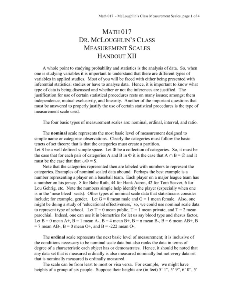
Math 017 - McLoughlin’s Class Measurement Scales, page 1 of 4
MATH 017
DR. MCLOUGHLIN’S CLASS
MEASUREMENT SCALES
HANDOUT XII
A whole point to studying probability and statistics is the analysis of data. So, when
one is studying variables it is important to understand that there are different types of
variables in applied studies. Most of you will be faced with either being presented with
inferential statistical studies or have to analyse data. Hence, it is important to know what
type of data is being discussed and whether or not the inferences are justified. The
justification for use of certain statistical procedures rests on many issues; amongst them
independence, mutual exclusivity, and linearity. Another of the important questions that
must be answered to properly justify the use of certain statistical procedures is the type of
measurement scale used.
The four basic types of measurement scales are: nominal, ordinal, interval, and ratio.
The nominal scale represents the most basic level of measurement designed to
simple name or categorise observations. Clearly the categories must follow the basic
tenets of set theory: that is that the categories must create a partition.
Let S be a well defined sample space. Let  be a collection of categories. So, it must be
the case that for each pair of categories A and B in  it is the case that A  B =  and it
must be the case that that  = S.
Note that the categories represented then are labeled with numbers to represent the
categories. Examples of nominal scaled data abound. Perhaps the best example is a
number representing a player on a baseball team. Each player on a major league team has
a number on his jersey. 8 for Babe Ruth, 44 for Hank Aaron, 42 for Tom Seaver, 6 for
Lou Gehrig, etc. Note the numbers simple help identify the player (especially when one
is in the ‘nose bleed’ seats). Other types of nominal scale data that statisticians consider
include; for example, gender. Let G = 0 mean male and G = 1 mean female. Also, one
might be doing a study of ‘educational effectiveness,’ so, we could use nominal scale data
to represent type of school. Let T = 0 mean public, T = 1 mean private, and T = 2 mean
parochial. Indeed, one can use it in biometrics for let us say blood type and rhesus factor,
Let B = 0 mean A+, B = 1 mean A-, B = 4 mean B+, B =  mean B-, B = 6 mean AB+, B
= 7 mean AB-, B = 0 mean O+, and B = -222 mean O-.
The ordinal scale represents the next basic level of measurement; it is inclusive of
the conditions necessary to be nominal scale data but also ranks the data in terms of
degree of a characteristic each object has or demonstrates. Hence, it should be noted that
any data set that is measured ordinally is also measured nominally but not every data set
that is nominally measured is ordinally measured.
The scale can be from least to most or visa versa. For example, we might have
heights of a group of six people. Suppose their heights are (in feet) 5’ 1”, 5’ 9”, 6’ 0”, 5’
Math 017- McLoughlin’s Class Measurement Scales, page 2 of 4
6”, 6’ 1”, and 6’ 2”. The scale might be the variable H1 such that h1 = 1 represents 5’ 1”,
h1 = 2 represents 5’ 9”, h1 = 3 represents 6’ 0”, h1 =4 represents 5’ 6”, h1 = 5 represents 6’
1”, and h1 = 6 represents 6’ 2”. So, H1 is simply nominal. However, if we define the
variable H2 such that h1 = 1 represents 5’ 1”, h2 = 3 represents 5’ 9”, h2 = 4 represents 6’
0”, h2 = 2 represents 5’ 6”, h2 = 5 represents 6’ 1”, and h2 = 6 represents 6’ 2” we have
constructed an ordinal scale. Note that this ordinal scale represents some sort of order
that (supposedly) is naturally occurring and accurate. The ordinal scale does not
necessarily measure such. Also, note that there is ranking but that the difference between
objects is not necessarily the same. Hence id we consider the scale difference we can see
this:
H2 = h2
Height
Difference in h2
Difference in height
1
5’ 1”
-
2
5’ 6”
1
5”
3
5’ 9”
1
3”
4
6’ 0”
1
3”
5
6’ 1”
1
1”
6
6’ 2”
1
1”
One might reasonably question the use of H2 and wonder why not just use the height. For
proper use, it would need to be converted to a measurement so that it is not as
complicated so we could define the interval scale H3 as height in inches so that we would
have:
Height
H3 = h3
5’ 1”
61
5’ 6”
66
5’ 9”
69
6’ 0”
72
6’ 1”
73
6’ 2”
74
The interval scale represents the next basic level of measurement; it is inclusive of
the conditions necessary to be nominal and ordinal scaled data but also includes the
condition that the data is ranked in measures that reflect equal distant predetermined
measures. So, the data is ranked and the degree of a characteristic each object has or
demonstrates is measured so that if the distance between x and y is 5 and the distance
between y and z is 5 the these distances are meaningful and the meaning is logically
equivalent. Most interval scales in use also have a zero point and have meaningful
negatives. Note that H3 from the previous example was measured on an interval scale.
With interval scaled data there is problem for researchers. The problem stems from
the fact that the interval scale does not imply that the equal distances between data mean
that there is a degree of ‘better’ that is clearly reflected or indeed that such really does
exist. For example, recall:
Height
H3 = h3
5’ 1”
61
5’ 6”
66
5’ 9”
69
6’ 0”
72
6’ 1”
73
6’ 2”
74
Does this mean that the 5’ 6” person is half (or some other such meaning) as tall as the 5’
9” person and likewise that the 5’ 9” person is half as tall as the 6’ 0” person? Is this 5’
9” person really exactly in the ‘middle’ of the other two? Of course not.
Math 017- McLoughlin’s Class Measurement Scales, page 3 of 4
Another interval scale that you are familiar with is grade point average (GPA) and
the grades assigned in schools. Note that we have the 4-point scale with the plus and the
minus.
Note that 0.0 is an ‘F,’ 1.0 is a ‘D,’ 2.0 is a ‘C,’ 3.0 is a ‘B,’ and 4.0 is an ‘A.’ Let us
ignore the illogical 4.0 also is an ‘A+’ for this discussion (for if we include it in the
discussion it clearly which renders this scale non-ordinal; hence, non-interval).
Consider the D and the C. Is a C twice as ‘acceptable’ as a D? Many seemingly make
this inference based on the numbers. So, they would conclude an A is ‘twice’ as ‘good’
as a C. Note the problem.
Other examples of interval scales are the degrees Fahrenheit, degrees Celsius, IQ
scores on the Stanford-Bitnet or Wechsler tests, and height in feet, meters, etc (which are
logically equivalent to the scale H3).
The ratio scale represents the ‘best’ basic level of measurement; it is inclusive of the
conditions necessary to be nominal, ordinal, and interval scaled data but also includes the
condition that there exists a true zero. For example, when one considers the scales of
degrees Fahrenheit and degrees Celsius one is faced with the problem of 0 F. and 0 C.
meaning two different things. Indeed when one considers that 40 F. and 40 C. are
radically different but -40 F. and -40 C. are the same one can see that these scales seem
arbitrary in some sort of way. However, when one considers the degrees Kelvin scale one
can see there does not exist (in a physical sense) negative degrees Kelvin; that -273 C. is
0 K. and that this absolute zero means that 80 K. is twice the temperature as 40 K;
whilst 160 K. is twice 80 K. so that a meaningful sense of ‘scale’ exists within the
confines of the degrees Kelvin.
The scale of time is also an example of a ratio scale such that we can use seconds (no
magic in this use minutes, hours, or some other such measure). The scale has an absolute
zero, has negatives and positives and is measurable (though not perfectly). Hence, the
existence of the absolute zero versus the arbitrary zero distinguishes the ratio from the
interval scale.
Math 017- McLoughlin’s Class Measurement Scales, page 4 of 4
Now, we are studying probability and statistics. We are considering random
variables as defined in handout 2, 3, and 5 as well as the book and other books. What we
have to determine when we are doing practical applications of the theory of probability
and statistics is to what degree can we adequately justify the statistics used and that
requires understanding the scale used. Returning to the baseball jersey discussion (3 for
Babe Ruth, 44 for Hank Aaron, 42 for Tom Seaver, 6 for Lou Gehrig) let us suppose we
put baseball cards in an urn such that each was equiprobable with the aforementioned
four players on each card. Let X be the player number. So, we have
X=x
Pr(X = x)
3
0.25
8
0.25
Now, calculating E[X] we get
42
0.25
44
0.25
 x  p (x) = 3  4  8  4  42  4  44  4 = 24.25.
1
1
1
1
x
x
This  is meaningless. It is nonsense. One can calculate it but in the practical application
work that most of you will do when you graduate (not if, when – get that idea and make it
a part of your subconscious) you have to consider this before doing statistical analyses.
So, a subject that one can study (post this course) is the types of measurement scales,
what statistics are proper for which type of scale, etc.
Cool, huh?
Last revised 2 March 2006
© 1994 – 2006 M. P. M. M. M.