5.73 Lecture #9
9–1
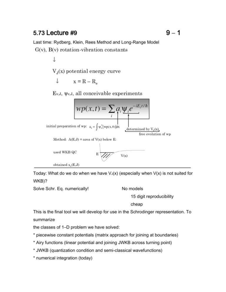
Last time: Rydberg, Klein, Rees Method and Long-Range Model
Today: What do we do when we have VJ(x) (especially when V(x) is not suited for
WKB)?
Solve Schr. Eq. numerically!
No models
15 digit reproducibility
cheap
This is the final tool we will develop for use in the Schrodinger representation. To
summarize
the classes of 1–D problem we have solved:
* piecewise constant potentials (matrix approach for joining at boundaries)
* Airy functions (linear potential and joining JWKB across turning point)
* JWKB (quantization condition and semi-classical wavefunctions)
* numerical integration (today)
5.73 Lecture #9
9–2
Numerical Integration of the 1-D Schrodinger Equation
widely used
incredibly accurate
no restrictions on V(x) or on E–V(x) [e.g. nonclassical region, near turning
points, double minimum potential, kinks in V(x).]
For most 1-D problems, where all one cares about is a set of {Ei,
}, where
is
See defined on a grid of points xi, one uses Numerov-Cooley
1. Cooley, Math. Comput. 15, 363 (1961).
2. Press et. al., Numerical Recipes, Chapters 16 and 17
Handouts
1. Classic unpublished paper by Zare and Cashion with listing of Fortran
program (now see LeRoy web site)
2. Tests of N-C vs. other methods by Tellinghuisen
Basic Idea: grid method
* solve differential equation by starting at some xi and propagating trial
solution from one grid point to the next
* apply
= 0 BCs at x = 0 and by two different tricks and then force
agreement at some intermediate point by adjusting E.
5.73 Lecture #9
Euler’s Method
want
(
at a series of grid points
is a number, not the entire wavefunction.)
For the Euler method, the generating function is simply:
For the Schrödinger Eqn.
9–3
5.73 Lecture #9
9–4
Schr. Eq. tells us the rule for propagating
. Employing Euler’s method (h is not
Planck’s constant):
in order to get things started we need two values of
edge of the region where
is defined and
starting at either
starts out very small.
See Press et. al. handout for discussion of nth-order Runge-Kutta
method. The generator is chosen more cleverly than in the
Euler method so that stepping errors are minimized by taking
more derivatives at intermediate points in the xi, xi+1 interval.
Cooley specifies
The result is that the error in yi1 is on the order of
— smaller error if h is smaller
(much better than Euler)
5.73 Lecture #9
So what do we do?
9–5
2 boundary conditions handled differently because we want
to define a finite # of equally spaced grid points (not
actually necessary — see Press: variable grid spacing which
is needed to sample infinite range of x with a finite number
of grid points)
use this to start the integration outward. If we have made
a wrong choice for
dividing all
, this can be corrected merely by
by an i-independent correction factor.
5.73 Lecture #9
At large R (the classically forbidden region), choose
9–6
at the last grid point, xn,
to be small and use WKB only once to compute the next to last grid point. We do
this because we have no reason to go to
• pre-exponential factors are approximately equal
• integrals in exponential factors are evaluated as summations
• in
, the common terms in the summations in the exponential factors
cancel
Once
is generated from
by JWKB, return to Cooley’s method of
numerical integration for all successive grid points.
So now we propagate one
from i = 0 out toward right and the
other one from i = n in toward the left. The “shooting” method.
5.73 Lecture #9
Stop the inward propagation of
9–7
when a point is reached where, for the first
time,
Since |
i|
at i=n until it reaches its first
is exponentially increasing from
maximum inside the classically allowed region, this outer lobe of
most important feature of
is also the
(because most of the probability resides in it).
Use outermost lobe because this is the global maximum of
(x), this minimizes
the problem of precision being limited by finite number of significant figures in the
computer.
Set value of
m=
From n,n-1,…m
(from the right)
From 0,1,…m
(from the left)
The renormalized
1.0 by renormalizing both functions
|
replace each
for all i down to m.
|
replace each
for all i up to m.
’s are denoted by
.
5.73 Lecture #9
9–8
This ensures that ψ(x) is continuous everywhere and that it satisfies grid form of
Schr. Eq. everywhere except i = m
In order to satisfy Schr. Eq. for i = m, it is necessary to adjust E. The above
equation can be viewed as a nonlinear requirement on E. At the crucial grid point i
= m, define an error function, F(E).
where we want to search for zeroes of F(E).
Assume that F(E) can be expanded about E1 (E1 is the initial, randomly chosen
value of E.)
and solve for the value of E where F(E) = 0.
Call this E2
5.73 Lecture #9
9-9
Usual approach: compute
Once the derivative is known, use it to compute correction to E1 (assuming
linearity).
Iterate until the correction,
criterion
, to E is smaller than a pre-set convergence
.
Now we have an eigenfunction of H and eigenvalue, E.
This procedure has been used and tested by many workers. A good version,
“Level 7.1” (schrq. f), is obtainable at Robert LeRoy’s web site:
http://theochem.uwaterloo.ca/~leroy/
I will assign some problems based on Numerov-Cooley method for integrating the
1-D Schr. Eq.