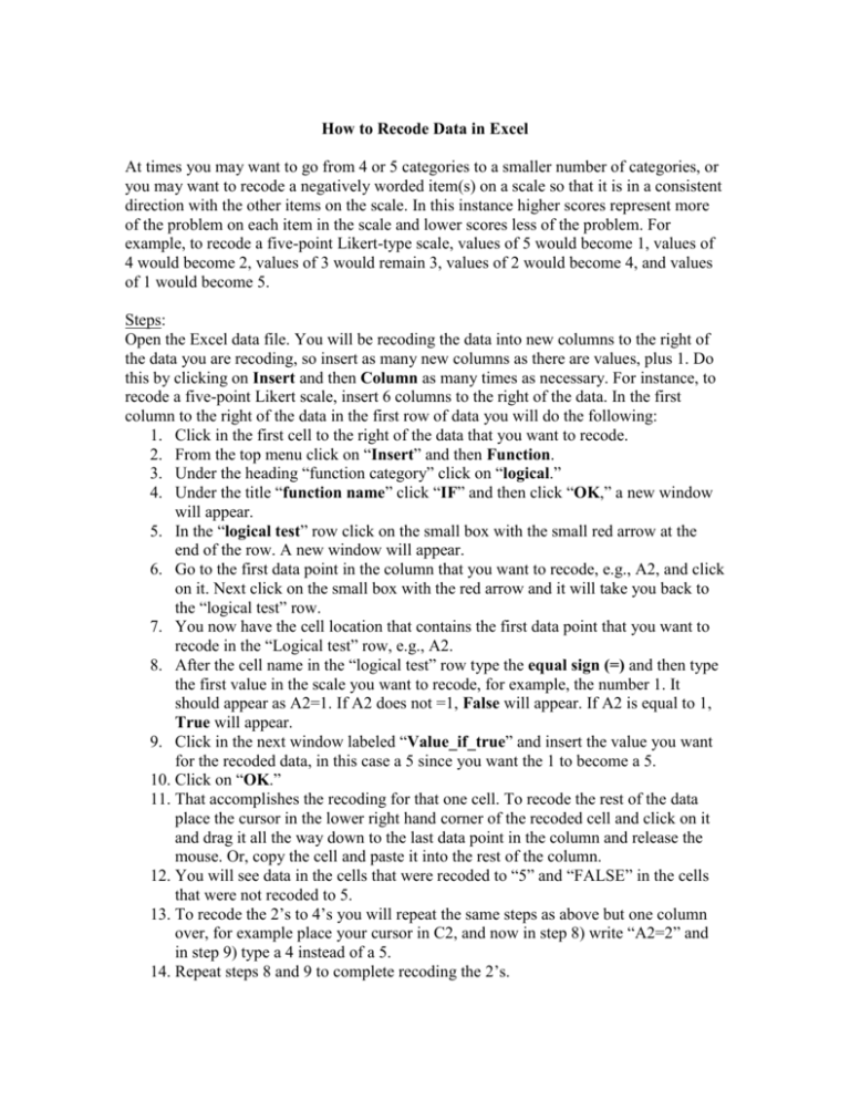
How to Recode Data in Excel
At times you may want to go from 4 or 5 categories to a smaller number of categories, or
you may want to recode a negatively worded item(s) on a scale so that it is in a consistent
direction with the other items on the scale. In this instance higher scores represent more
of the problem on each item in the scale and lower scores less of the problem. For
example, to recode a five-point Likert-type scale, values of 5 would become 1, values of
4 would become 2, values of 3 would remain 3, values of 2 would become 4, and values
of 1 would become 5.
Steps:
Open the Excel data file. You will be recoding the data into new columns to the right of
the data you are recoding, so insert as many new columns as there are values, plus 1. Do
this by clicking on Insert and then Column as many times as necessary. For instance, to
recode a five-point Likert scale, insert 6 columns to the right of the data. In the first
column to the right of the data in the first row of data you will do the following:
1. Click in the first cell to the right of the data that you want to recode.
2. From the top menu click on “Insert” and then Function.
3. Under the heading “function category” click on “logical.”
4. Under the title “function name” click “IF” and then click “OK,” a new window
will appear.
5. In the “logical test” row click on the small box with the small red arrow at the
end of the row. A new window will appear.
6. Go to the first data point in the column that you want to recode, e.g., A2, and click
on it. Next click on the small box with the red arrow and it will take you back to
the “logical test” row.
7. You now have the cell location that contains the first data point that you want to
recode in the “Logical test” row, e.g., A2.
8. After the cell name in the “logical test” row type the equal sign (=) and then type
the first value in the scale you want to recode, for example, the number 1. It
should appear as A2=1. If A2 does not =1, False will appear. If A2 is equal to 1,
True will appear.
9. Click in the next window labeled “Value_if_true” and insert the value you want
for the recoded data, in this case a 5 since you want the 1 to become a 5.
10. Click on “OK.”
11. That accomplishes the recoding for that one cell. To recode the rest of the data
place the cursor in the lower right hand corner of the recoded cell and click on it
and drag it all the way down to the last data point in the column and release the
mouse. Or, copy the cell and paste it into the rest of the column.
12. You will see data in the cells that were recoded to “5” and “FALSE” in the cells
that were not recoded to 5.
13. To recode the 2’s to 4’s you will repeat the same steps as above but one column
over, for example place your cursor in C2, and now in step 8) write “A2=2” and
in step 9) type a 4 instead of a 5.
14. Repeat steps 8 and 9 to complete recoding the 2’s.
15. If your scale has an odd number of values such as in a five-point scale the middle
value will be recoded into the same number. To recode the 3s write “B2=3” and
then enter a 3 for the new value.
16. To recode the 4’s write “B2=4” and a 2 for the new value.
17. To recode the 5s write “B2=5” and a 1 for the new value.
18. The last step is to put all the data in a single column. So in a column one over
from the last recoded value click in the first cell and sum the columns with the
recoded data. Say that the original data is in “A2”, the first recoded data is in
“B2”, “C2”, “D2”, “E2”, and “F2”. In “H2” write by clicking in the cell and then
typing “=B2+C2+D2+E2+F2” and then pressing “Enter.”
19. Then click with the mouse on the lower right corner of the cell and drag it all the
way down to the last data point. Release the mouse and you are done. Or, use
Copy/Paste to copy the contents of the cell to the entire column. This column
contains the recoded data.