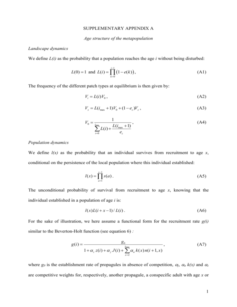
SUPPLEMENTARY APPENDIX A
Age structure of the metapopulation
Landscape dynamics
We define L(i) as the probability that a population reaches the age i without being disturbed:
i 1
L(0)  1 and L(i )   1  e( k )  ,
(A1)
k 0
The frequency of the different patch types at equilibrium is then given by:
Vi  L(i)V0 ,
(A2)
Vz  L(imax  1)V0  (1  ez )Vz ,
(A3)
V0 
1
,
L(imax  1)
L(i) 

ez
i 0
(A4)
imax
Population dynamics
We define l(x) as the probability that an individual survives from recruitment to age x,
conditional on the persistence of the local population where this individual established:
x 1
l ( x)   s (a ) .
(A5)
a 1
The unconditional probability of survival from recruitment to age x, knowing that the
individual established in a population of age i is:
l ( x) L(i  x  1) / L(i ) .
(A6)
For the sake of illustration, we here assume a functional form for the recruitment rate g(i)
similar to the Beverton-Holt function (see equation 6) :
g (i ) 
g0
xmax
1   z z (i )   j J (i )    a k ( x ) n(i  1, x )
,
(A7)
x 2
where g0 is the establishment rate of propagules in absence of competition, j, a k(x) and z
are competitive weights for, respectively, another propagule, a conspecific adult with age x or
1
a member of the competitively superior species. The following recursions could however be
achieved using any functional form for the juvenile survival by replacing the expression for
g(i) when necessary.
The number of individuals in each age class is computed by recurrence, by fixing an initial
value for J(0)t the number of immigrants in an empty patch and using the following relations:
g (0)t 
g0
1   z z(0)   j J (0)t
(A8)
n(1,1)t  J (0)t g  0t and for all x  1 n(1, x)  0
(A9)
n(i  1, x  1)t  s( x)n(i, x)t
(A10)
xmax
J (i )t  J (0)t   n(i, x)t f ( x) 1  d (i ) 
(A11)
x 1
g (i ) t 
g0
xmax
1   z z (i )   j J (i )t    a k ( x ) n(i  1, x )t
(A12)
x 2
n(i  1,1)t  J (i )t g (i )t
(A13)
A new value for the number of immigrants J(0)t+1 can then be computed from the n(i,x)t
imax xmax
J (0)t 1  (1  c)Vi n(i, x)t f ( x)d (i )
(A14)
i 1 x 1
Such computation was iterated until we converged to a fixed value for J(0).
2