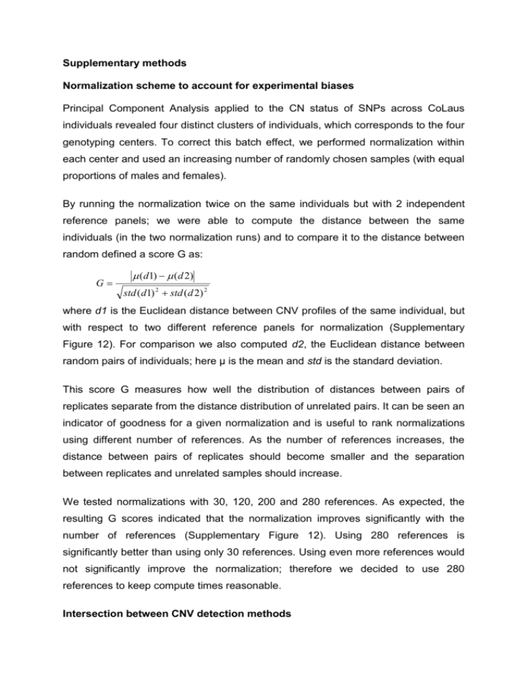
Supplementary methods
Normalization scheme to account for experimental biases
Principal Component Analysis applied to the CN status of SNPs across CoLaus
individuals revealed four distinct clusters of individuals, which corresponds to the four
genotyping centers. To correct this batch effect, we performed normalization within
each center and used an increasing number of randomly chosen samples (with equal
proportions of males and females).
By running the normalization twice on the same individuals but with 2 independent
reference panels; we were able to compute the distance between the same
individuals (in the two normalization runs) and to compare it to the distance between
random defined a score G as:
G
 (d1)   (d 2)
std (d1) 2  std (d 2) 2
where d1 is the Euclidean distance between CNV profiles of the same individual, but
with respect to two different reference panels for normalization (Supplementary
Figure 12). For comparison we also computed d2, the Euclidean distance between
random pairs of individuals; here µ is the mean and std is the standard deviation.
This score G measures how well the distribution of distances between pairs of
replicates separate from the distance distribution of unrelated pairs. It can be seen an
indicator of goodness for a given normalization and is useful to rank normalizations
using different number of references. As the number of references increases, the
distance between pairs of replicates should become smaller and the separation
between replicates and unrelated samples should increase.
We tested normalizations with 30, 120, 200 and 280 references. As expected, the
resulting G scores indicated that the normalization improves significantly with the
number of references (Supplementary Figure 12). Using 280 references is
significantly better than using only 30 references. Using even more references would
not significantly improve the normalization; therefore we decided to use 280
references to keep compute times reasonable.
Intersection between CNV detection methods
Overlap-based approaches are useful to compare the CNV predictions between two
distinct methods. But it becomes tedious when comparing results between more than
two methods. A way to simplify this problem is to use a common number of elements
to compare between the different methods. The full autosomal dataset was subjected
to “LD based pruning”, as implemented in plink (Purcell S et al. 2007). We used a
sliding window of 100 SNPs, sliding along in 20 SNP increments. SNPs with a
variance inflation factor (VIF) greater than 1.2 were pruned from each window. This
procedure identified around 60’000 autosomal SNPs. Then, for each method, we
created a binary SNP vector, indicating which SNPs where found variant (‘non-copy
neutral’) or copy neutral in the CoLaus population. This facilitates the comparison and
the number of SNPs found variant in one or more methods can easily be computed.
We used such approach both for pair-wise comparison (reporting the Jaccard index
between non-copy neutral SNPs) and for generating 4-way Venn diagrams (reporting
the number of concordant non-copy neutral predictions between methods).
Comparisons were made using 1) all 60’000 SNPs, 2) using SNPs with CNV
frequency greater than 1% (referred as ‘CNPs’) and 3) using SNPs with CNV
frequency less than 1% (‘rare CNVs’).
Evaluation of the Gaussian Mixture Model using simulated data
To evaluate the true and false positive rates of our Gaussian Mixture Model, we
generated an artificial dataset composed of 5600 individuals, in which the true copy
number status was defined and different levels of Gaussian noise was added. This
approach is similar to other studies (Lai WR et al. 2005, Willenbrock H and Fridlyand
J 2005). In more details, our artificial dataset consists of a distribution of log 2 ratios
(n=5600), where a predefined number of individuals should reflect a deletion state
(log2 ratio = -1); all remaining individuals are copy neutral thus log2 ratios = 0. We
then added Gaussian noise to the true copy numbers and tested the ability of our
model to correctly detect the underlying copy number state. Supplementary Figure 17
illustrates one test where half of the population is expected to have a deletion.
Supplementary figure 18 shows the performance of our model as a function of the
number of individuals sharing the CNV. Each colored curve corresponds to a different
level of noise in the data (from low : σ=0.1 to high : σ=0.6). This analysis was
repeated 50 times for each point of the curves (mean and standard deviation are
shown in the figure). The high TPR and very low FPR demonstrate the good
performance of our model.
SNP clustering using Self-Organizing Maps
Self-organizing map (SOM) is a form of artificial neural network, where the network
learns from the data and can perform discrete clustering on the same (learning)
dataset. Neural networks are made with nodes (neurons) positioned in the space (a
map). Such maps are usually hexagonal or rectangular grids, made with neurons that
can connect to their neighbors. Connections between neurons are defined by their
distance and by their weights computed from the data. The weight defines the neuron
position in the map and is adjusted in a learning phase. This re-adjustment further
refines the neuron position and following the learning phase, neurons with similar
weights define a same cluster. A specificity of SOMs, by contrast to competitive
layers, is that not only the weight from the winning neuron (i.e. the one with weight
the closest to the data) but the weight from all neurons in a given neighborhood is
updated.
In our analysis, the network is a hexagonal grid of 5 by 3 neurons and is initialized
with the newsom Matlab function (Neural Network toolbox). The input vectors are
defined by the 'SNP' eigen-vectors resulting from the projection on Principal
Components that explain up to 90% of the variance. Subsequently to the training
phase, clustering of SNPs is achieved by assigning them the nearest neuron of the
SOM. SNPs that belong to the same cluster and that are physically adjacent are
merged into the same CNVR.
Since performing a PCA analysis genome-wide or chromosome wise is
computationally intensive, we define "blocks of copy number variation" as a
chromosomal region flanked with two regions, both with a length greater than a userspecified threshold (e.g. 1Mb) and where all SNPs for all individuals were predicted
with the diploid state (CN=2). For each of these blocks, we apply our PCA merging
procedure and obtain CNVRs made of SNPs that explain the variance in a similar
fashion (i.e. similar pattern of eigen-values).
Supplementary Figures
Supplementary Figure 1 Simple merge illustration
A Illustration of the simple merge. Data for each chromosome can be represented as
a matrix individual (rows) by SNPs (columns). Each matrix element corresponds to
the discrete copy number. SNPs are sorted by genomic position. The simple merge
consists in merging strictly identical columns into region. In this illustration, the
resulting regions would be columns having the same color. B Simple merge (red
segments) applied on a local SNP window (chromosome3:74.5-76.5Mb) across
CoLaus individual. Regions in red regions obtained from simple merge and in blue,
regions from the PCA merge. The Y axis represents CNV frequency in the CoLaus
population (n≈5600)
Supplementary Figure 2 Merging SNPs into CNVs using principal component
analysis
Top plot shows a principal component analysis (PCA) on a local SNP window
(chromosome3:74.5-76.5Mb) across CoLaus individual. The main components are
on Y axis and adjacent SNPs are on X axis. The bottom plot shows in red regions
obtained from simple merge and in blue, regions from the PCA merge. The Y axis
represents CNV frequency in the CoLaus population (n≈5600).
Supplementary Figure 3 Number of CNVs per method
The Y axis indicates the number (log10) of CNPs or CNVRs for each combination of
a given CNV detection method method (CBS, CNAT.allelic, CNAT.total or GMM) and
merge approach (simpleMerge or pcaMerge). Statistics are provided for each
autosome (chromosome 1 to 22) and for all autosomal chromosomes together
(chromosome 0).
Supplementary Figure 4 Distribution of the CNV length per method and for
common (CNPs) and rare (CNVRs) variants
Variants are classified according to their length: single-SNP (1bp), size greater than
1bp and less than 1Kb, size greater or equal than 1Kb. Title from each panel
indicates the CNV detection method (CBS, CNAT.allelic, CNAT.total or GMM) and
the CNV frequency class (CNPs or CNVRs). Statistics are provided for each
autosome (chromosome 1 to 22) and for all autosomal chromosomes together
(chromosome 0).
Supplementary Figure 5 Percentage of chromosome covered with common
(CNPs) or rare (CNVRs) variants
The Y axis indicates the % of a chromosome that is covered with CNPs or CNVRs for
each combination of a given CNV detection method method (CBS, CNAT.allelic,
CNAT.total or GMM) and merge approach (simpleMerge or pcaMerge). Statistics are
provided for each autosome (chromosome 1 to 22) and for all autosomal
chromosomes together (chromosome 0).
Supplementary Figure 6 CNV frequency on chromosome 1
Each plot shows the CNV prediction from a CNV detection algorithm (title indicates
the method name). Each cyan bars is a SNP on chromosome 1, the bar height
represent the % of CoLaus individuals found as having this SNP as variant (deleted
or duplicated). In red are regions defined by the PCA merge, the height shows the
maximal CNV frequency found in this region. Only regions with CNV frequency
greater than 0.1% are plotted.
CBS
CNAT.allelic
CBS
GMM
CNAT.allelic
GMM
8738
6925
3874
8027
2692
CNAT.total
619
2659
490
42
2202
547
24
34
91
242
1044
CNAT.total
75
28
3834
1922
195
276
2815
3188
767
5
241
3
10
3
CNPs
rare CNVs
CBS
CNAT.allelic
GMM
4648
7312
6632
8693
2811
CNAT.total
394
111
3726
1673
6064
2375
390
615
280
86
All CNVs
Supplementary Figure 7 Intersection between CNVs methods
Intersection between the different CNV detection methods using the CNV status at
60k autosomal and independent SNP (i.e. SNPs that are not in LD in the CEU
population). The percentage of SNPs found variant in several methods is indicated in
Supplementary Table 3.
Overlap between Affymetrix CNVRs and published CNVs
p<1E-3
p<1E-3
p=0.002
p<1E-3
p=0.002
p<1E-3
10
p<1E-3
2
p<1E-3
p=0.385
p<1E-3
p=0.060
p<1E-3
p<1E-3
p<1E-3
GMM
CBS
CNAT.allelic
CNAT.total
p<1E-3
3
10
p<1E-3
p<1E-3
p<1E-3
p=0.005
p<1E-3
4
10
number of regions
p=0.003
1
p<1E-3
p<1E-3
p<1E-3
p<1E-3
p<1E-3
p<1E-3
p=0.367
p=0.012
p<1E-3
p<1E-3
p=0.062
p<1E-3
2
10
p=0.453
p=0.057
p<1E-3
p=0.478
10
p<1E-3
number of regions
3
GMM
CBS
CNAT.allelic
CNAT.total
p<1E-3
4
10
p<1E-3
Overlap between Affymetrix CNPs and published CNVs
1
10
10
0
10
0
0
0
]0-25]
]25-50]
Overlap (%)
]50-75]
]75-100]
]75-100]
p<1E-3
p=0.043
0
10
p<1E-3
p<1E-3
p=0.064
p=0.006
1
10
p=0.004
p=0.265
p<1E-3
p<1E-3
p<1E-3
2
10
p=0.480
number of regions
3
10
GMM
CBS
CNAT.allelic
CNAT.total
p<1E-3
4
10
p=0.256
p=0.007
p<1E-3
0
10
p=0.025
p<1E-3
p=0.342
p<1E-3
p<1E-3
p=0.110
p<1E-3
p=0.013
1
10
p<1E-3
p<1E-3
p<1E-3
p<1E-3
p<1E-3
p<1E-3
p<1E-3
number of regions
2
10
]50-75]
Overlap between Affymetric CNVRs and Illumina CNVs
GMM
CBS
CNAT.allelic
CNAT.total
p<1E-3
p<1E-3
p<1E-3
3
]25-50]
Overlap (%)
Overlap
(%) and Illumina CNVs
Overlap between Affymetrix
CNPs
10
]0-25]
]75-100]
p<1E-3
]50-75]
p=0.311
]25-50]
p<1E-3
]0-25]
p<1E-3
0
p<1E-3
10
0
]0-25]
]25-50]
]50-75]
Overlap (%)
Supplementary Figure 8 Overlap between CNPs/CNVRs and published
CNVs/Illumina CNVs
These figures are similar to figures two and three. Each plot title indicates the overlap
analysis. Overlap is measured by the Jacquard coefficient, i.e. the ratio between the
intersect and the union of two CNVs. Expected counts from reshuffled data (n=1000)
are shown in gray (extending over one standard deviation). Estimated p-values are
indicated for significant enrichment (red) or depletion (blue), with respect to these
controls. Non significant p-values (alpha>1%) are shown in black.
]75-100]
Supplementary Figure 9 Rank comparison of Precision-Recall AUCs when predicting relatedness using all CNPs
(frequency >= 1% and no size filter)
Rank comparison (Kruskal–Wallis test) of the performance, from different CNV methods, at predicting relatedness between
subjects. Performance was measured as the Precision-Recall AUCs and analyses were re-iterated 100 times with randomly chosen
pairs of unrelated individuals. Method names are indicated in the X axis, those used in combination of the ‘PCA merge’ and ‘simple
merge’ are shown respectively in blue and red. Dots correspond to the mean group rank and bars indicate the comparison interval.
Groups with non-overlapping intervals are significantly different (P-values were adjusted for multiple testing issues using a
Bonferroni correction, where the number of tests is the number of pairwise comparisons; the resulting adjusted P-value was less
than 0.05).
Supplementary Figure 10 Boxplot representation of Precision-Recall AUCs
when predicting relatedness using all CNPs (frequency >= 1% and no size
filter)
Boxplot representation of the performance from different CNV methods at predicting
relatedness between subjects. Performance was measured as the Precision-Recall
AUCs and analyses were re-iterated 100 times with randomly chosen pairs of
unrelated individuals. Method names are indicated in the X axis, those used in
combination of the ‘PCA merge’ and ‘simple merge’ are respectively shown in blue
and red.
Supplementary Figure 11 Check for genotyping center bias with the initial data
normalization
PCA analysis using copy number ratios normalized using a reference panel of 30
CoLaus individuals. Each dot represent an individual, color indicates in which
genotyping center, the sample was processed. Top panel shows the first and second
main components, bottom panel shows first and third components.
Supplementary Figure 12 Improvement of the normalization as a function of the
reference panel size
In cyan are shown the distances (n=55) between the CNV profiles as predicted by
two independent reference panel (having the same size) for a same individual. In red
are the distances between unrelated individuals predicted by these two reference
panels. Different size of reference panel have been tested (30,120,200 and 280). The
T’ score is an estimate of the separation between pairs of identical individuals (same)
and controls and is computed as:
T'
abs (mean( same)  mean(controls ))
std ( same) 2  std (controls ) 2
Supplementary Figure 13 Check for genotyping center bias subsequently to
data renormalization
PCA analysis using copy number ratios normalized using a reference panel of 280
CoLaus individuals (with samples from both test and reference panel matched for the
genotyping center). Each dot represent an individual, color indicates in which
genotyping center, the sample was processed. Top panel shows the first and second
main components, bottom panel shows first and third components.
Supplementary Figure 14 Check for SNP array (NSP/STY) bias subsequently to
data renormalization
PCA analysis using copy number ratios normalized using a reference panel of 280
CoLaus individuals (with samples from both test and reference panel matched for the
genotyping center). Each dot represent a SNP, color indicates on which array the
SNP was assayed. Top panel shows the first and second main components, bottom
panel shows first and third components.
3
3
2
2
1
1
0.25
0
-0.25
0.25
0
-0.25
-1
-1
-2
-2
-3
-3
-4
-4
-5
-5
-6
1
-6
0
2
4
6
8
4
x 10
Supplementary Figure 15 Distribution of CBS segment mean ratios
Distribution of all CBS segments mean log2 ratios, detected in the 5612 CoLaus
individuals. Left panel shows a boxplot representation. Median is -0.007 (and mean 0.0637), inter-quartile 0.114 and 25th and 75th percentiles are respectively -0.082 and
0.032. Right panel shows an histogram representation, data have been clustered
using a 3 components Gaussian Mixture Model (color indicates data points from a
same cluster).
Histogram of log2 ratio for 5613 individuals at a single SNP
700
600
500
400
300
200
100
0
-3
-2.5
-2
-1.5
-1
-0.5
0
0.5
1
Probabilities to belong to a given CN state
1
individuals
1000
0.8
2000
0.6
3000
0.4
4000
0.2
5000
1
2
3
4
0
CN state
Supplementary Figure 16 CNV calling using Gaussian Mixture Model
Top panel, distribution of log2 ratios for all 5613 CoLaus individuals at a single SNP.
Bottom panel, matrix of probabilities for CoLaus individuals to have the queried SNP
in a deletion state (CN=1), copy neutral (CN=2), with one or additional copy (CN=3
4
and CN=4). The CN dosage value can be computed as i 1 Pi * Ci where Pi
represents the probability at an individual j and a SNP k to be in the copy number
state Ci.
Distribution of log2 ratios (n=5600 individuals , noise variance = 0.20)
140
A
120
100
80
60
40
20
-2.5
-2
-1.5
-1
Probabilities per CN component
individuals
1000
2000
0.6
3000
0.4
4000
0.5
D
1.8
2000
1.6
3000
1.4
4000
0.2
5000
1
1.5
Truth
2
1000
0.8
0
CN value
C
individuals
B
-0.5
1.2
CNV
2507
485
293
2315
CNV
neutral
Predicted
0
-3
neutral
5000
1
2
3
4
truth pred.
1
CN
Supplementary Figure 17 Testing the Gaussian Mixture Model on simulated
data
A Distribution of simulated log2 ratios (n=5600) with Gaussian noise (σ=0.2). Half of
the individuals have an underlying log2 ratio = -1 (deletion) and the remaining log2
ratio = 0 (copy neutral) B Probabilities, as computed by our Gaussian Mixture Model,
for each individual (Y axis) to belong to a given copy number state (X axis) C
Comparison between the true and predicted copy number state of each individual D
Contingency table containing the number of individuals correctly or incorrectly
predicted.
TPR
1
0.8
0.1
0.2
0.4
0.6
0.6
6
17
28
45
56
112
280
560
1120
2240
3360
6
17
28
45
56
112
280
560
1120
2240
3360
6
17
28
45
560
1120
2240
3360
FDR
0.4
0.2
0
0.03
FPR
0.02
0.01
0
56
112
280
CNV frequency (#inds)
Supplementary Figure 18 Performance of the Gaussian Mixture Model
Panels show respectively from top to bottom, the True Positive, False Discovery and
False Positive rates, when predicting deletions (with predefined frequency, see X
axis) in a population of n=5600 individuals. The different curves correspond to
simulated data with a given Gaussian noise (see graph legend). Each point is the
mean from 50 resamplings, error bars correspond to one standard deviation.
Supplementary tables
GMM
CBS
CNAT.allelic
CNAT.total
PCA merged
CNPs
CNVRs
2.4
9.86
1.54
42.43
12.4
30.88
0.73
12.71
Simple merge
CNPs
CNVRs
0.02
0.38
0.09
24.23
8.08
21.19
0.15
7.79
Supplementary Table 1 genome (autosomal chromosomes) coverage of CNVs
identified by different methods
CNV detection methods are shown as rows, the merging approach as columns.
Distinction is made between CNPs (i.e. CNVs with population frequency above 1%)
and CNVRs (i.e. CNVs with population frequency below 1% but seen for at least five
individuals). The coverage is expressed as the % of the autosomes.
CNPs
% of SNPs found variant in at least 3
methods
2.3
% of SNPs found variant in at least 2
methods
10
CNVRs
All CNVs
23.5
27.21
55.3
59.17
Supplementary Table 2 Percentage of SNPs found copy number variant by
several methods
CNPS
GMM
CBS
CNAT.allelic
CNAT.total
GMM
3226 (100.00%)
CNVRs
GMM
CBS
CNAT.allelic
CBS
317 (8.00%)
1055 (100.00%)
CNAT.allelic
366 (5.58%)
228 (5.03%)
3705 (100.00%)
CNAT.total
102 (3.06%)
138 (12.22%)
172 (4.59%)
212 (100.00%)
GMM
CBS
25355 (100.00%) 15720 (39.54%)
30119 (100.00%)
CNAT.allelic
9118 (26.34%)
11543 (31.24%)
18376 (100.00%)
CNAT.total
5666 (19.48%)
7847 (24.78%)
7073 (34.16%)
9401
(100.00%)
GMM
CBS
28581 (100.00%) 19098 (46.97%)
31174 (100.00%)
CNAT.allelic
12555 (32.95%)
14274 (36.62%)
22081 (100.00%)
CNAT.total
7155 (23.05%)
8632 (26.84%)
8521 (36.77%)
9613
(100.00%)
CNAT.total
ALL CNVs
GMM
CBS
CNAT.allelic
CNAT.total
Supplementary Table 3 Pairwise comparison between CNV detection methods
Pairwise comparison between the different detection methods using the CNV status
at 60k autosomal and independent SNPs (i.e. SNPs that are not in LD in the CEU
population). Intersection is reported as the number of SNPs found variant in both
methods, the percentage, indicated between the parentheses, corresponds to the
intersection divided by the union of SNPs found variant in any of the two methods.
The number of variant SNPs in each method (independently of any other methods) is
indicated as self-self comparison.
0
]0-25]
]25-50]
]50-75]
]75-100]
GMM
-12.21
8.79
7.53
7.25
9.48
CBS
-10.26
6.27
4.75
4.15
13.75
CNAT.allelic
-3.62
1.20
0.81
3.17
7.03
CNAT.allelic
-10.42
6.36
4.12
6.25
11.43
Supplementary Table 4 T statistic values for overlap between CNVs identified
from CoLaus and published CNVs
The T statistic is computed from the difference between observed overlap and
expected counts normalized by the standard deviation of expected counts. Expected
counts are inferred from the overlap between reshuffled data (n=1000) and published
CNVs. T statistics greater than 2.58 are significant with α=1%. Positive (negative) T
statistics indicates enrichment (depletion) with respect to the expected counts.
0
]0-25]
]25-50]
]50-75]
]75-100]
GMM
-17.68
12.14
12.81
5.49
15.14
CBS
-12.67
9.78
8.45
12.28
6.13
CNAT.allelic
0.31
-1.01
1.06
1.95
0.34
CNAT.allelic
-9.69
6.81
8.59
7.78
7.18
Supplementary Table 5 T statistic values for overlap between CNVs identified
from Affymetrix and Illumina data
The T statistic is computed from the difference between observed overlap and
expected counts normalized by the standard deviation of expected counts. Expected
counts are inferred from the overlap between reshuffled data (n=1000) and CNVs
identified on Illumina. T statistics greater than 2.58 are significant with α=1%. Positive
(negative) T statistics indicates enrichment (depletion) with respect to the expected
counts.