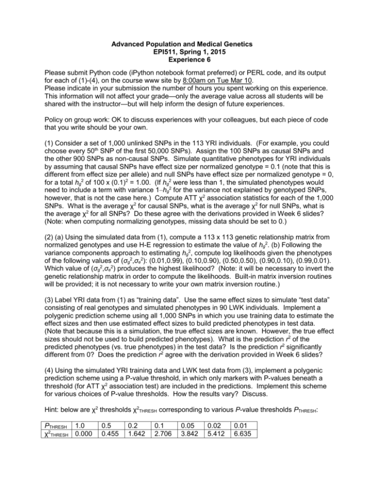
Advanced Population and Medical Genetics
EPI511, Spring 1, 2015
Experience 6
Please submit Python code (iPython notebook format preferred) or PERL code, and its output
for each of (1)-(4), on the course www site by 8:00am on Tue Mar 10.
Please indicate in your submission the number of hours you spent working on this experience.
This information will not affect your grade—only the average value across all students will be
shared with the instructor—but will help inform the design of future experiences.
Policy on group work: OK to discuss experiences with your colleagues, but each piece of code
that you write should be your own.
(1) Consider a set of 1,000 unlinked SNPs in the 113 YRI individuals. (For example, you could
choose every 50th SNP of the first 50,000 SNPs). Assign the 100 SNPs as causal SNPs and
the other 900 SNPs as non-causal SNPs. Simulate quantitative phenotypes for YRI individuals
by assuming that causal SNPs have effect size per normalized genotype = 0.1 (note that this is
different from effect size per allele) and null SNPs have effect size per normalized genotype = 0,
for a total hg2 of 100 x (0.1)2 = 1.00. (If hg2 were less than 1, the simulated phenotypes would
need to include a term with variance 1–hg2 for the variance not explained by genotyped SNPs,
however, that is not the case here.) Compute ATT χ2 association statistics for each of the 1,000
SNPs. What is the average χ2 for causal SNPs, what is the average χ2 for null SNPs, what is
the average χ2 for all SNPs? Do these agree with the derivations provided in Week 6 slides?
(Note: when computing normalizing genotypes, missing data should be set to 0.)
(2) (a) Using the simulated data from (1), compute a 113 x 113 genetic relationship matrix from
normalized genotypes and use H-E regression to estimate the value of hg2. (b) Following the
variance components approach to estimating hg2, compute log likelihoods given the phenotypes
of the following values of (σg2,σe2): (0.01,0.99), (0.10,0.90), (0.50,0.50), (0.90,0.10), (0.99,0.01).
Which value of (σg2,σe2) produces the highest likelihood? (Note: it will be necessary to invert the
genetic relationship matrix in order to compute the likelihoods. Built-in matrix inversion routines
will be provided; it is not necessary to write your own matrix inversion routine.)
(3) Label YRI data from (1) as “training data”. Use the same effect sizes to simulate “test data”
consisting of real genotypes and simulated phenotypes in 90 LWK individuals. Implement a
polygenic prediction scheme using all 1,000 SNPs in which you use training data to estimate the
effect sizes and then use estimated effect sizes to build predicted phenotypes in test data.
(Note that because this is a simulation, the true effect sizes are known. However, the true effect
sizes should not be used to build predicted phenotypes). What is the prediction r2 of the
predicted phenotypes (vs. true phenotypes) in the test data? Is the prediction r2 significantly
different from 0? Does the prediction r2 agree with the derivation provided in Week 6 slides?
(4) Using the simulated YRI training data and LWK test data from (3), implement a polygenic
prediction scheme using a P-value threshold, in which only markers with P-values beneath a
threshold (for ATT χ2 association test) are included in the predictions. Implement this scheme
for various choices of P-value thresholds. How the results vary? Discuss.
Hint: below are χ2 thresholds χ2THRESH corresponding to various P-value thresholds PTHRESH:
PTHRESH 1.0
χ2THRESH 0.000
0.5
0.455
0.2
1.642
0.1
2.706
0.05
3.842
0.02
5.412
0.01
6.635
Possible topics for short Research Paper (an aggregate list of suggested topics will be provided
on Feb 24. At that time, each student should choose one topic from the aggregate list.):
• Use HapMap3 data from diverse populations to compare and contrast three different strategies
for conducting polygenic prediction in a target population when the only training data available is
from a population with different continental ancestry than the target population. The first
strategy is polygenic prediction with a P-value threshold (see Experience 6). The second
strategy is LD-pruning (remove one of each pair of nearby markers that are in strong LD)
followed by polygenic prediction with a P-value threshold. The third strategy is a strategy
different from the second strategy that is informed by LD in the training data. Discuss how
results vary when the training population has either more or less LD than the target population.
Compare to results that can be achieved when the training and target population are the same.
• Or, feel free to design your own research topic.