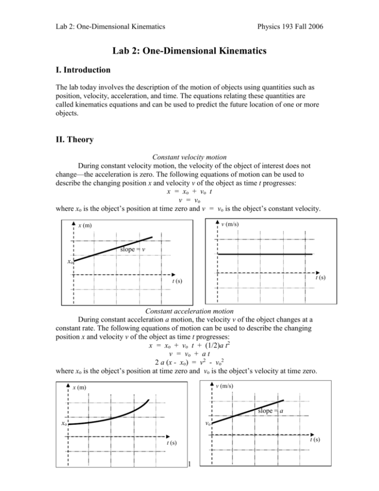
Lab 2: One-Dimensional Kinematics
Physics 193 Fall 2006
Lab 2: One-Dimensional Kinematics
I. Introduction
The lab today involves the description of the motion of objects using quantities such as
position, velocity, acceleration, and time. The equations relating these quantities are
called kinematics equations and can be used to predict the future location of one or more
objects.
II. Theory
Constant velocity motion
During constant velocity motion, the velocity of the object of interest does not
change—the acceleration is zero. The following equations of motion can be used to
describe the changing position x and velocity v of the object as time t progresses:
x = xo + vo t
v = vo
where xo is the object’s position at time zero and v = vo is the object’s constant velocity.
v (m/s)
x (m)
slope = v
xo
t (s)
t (s)
Constant acceleration motion
During constant acceleration a motion, the velocity v of the object changes at a
constant rate. The following equations of motion can be used to describe the changing
position x and velocity v of the object as time t progresses:
x = xo + vo t + (1/2)a t2
v = vo + a t
2 a (x - xo) = v2 - vo2
where xo is the object’s position at time zero and vo is the object’s velocity at time zero.
v (m/s)
x (m)
slope = a
vo
xo
t (s)
t (s)
1
Lab 2: One-Dimensional Kinematics
Physics 193 Fall 2006
III. Experiments
Using a Motion Detector to Measure Motion
Read the write-up on how to use Logger Pro that is taped next to the computers.
We will use a motion detector to produce position-versus-time and velocity-versus-time
graphs of the motion of a dynamics cart on a track. The motion detector can record the
cart’s position if farther than about 0.5 m from the detector and if closer than about 2 or 3
meters from the detector. You have to be careful that the motion detector is not
measuring the position of some other object than the intended object—keep other things
out of the region in front of the detector. Be sure the track is level and clean (to reduce
friction).
Experiment 1a—constant velocity in positive direction: Place the cart about 0.5 meters
from the detector and give it a gentle push. Then release the cart so that it glides slowly
away from the detector. If moving at constant velocity, the position-versus-time graph
should look something like shown in (a) below and the velocity-versus-time graph should
look like that shown in (b). Do the graphs look like those shown below? If not, why not?
Repeat the motion, only push the cart a little harder so that it glides at a faster initial
velocity. In (c) and (d) below, draw a position-versus-time graph and a velocity-versustime graph for this observed motion when starting at a faster velocity away from the
detector.
(a)
(b)
v (m/s)
x (m)
slope = v
xo
t (s)
t (s)
(c)
(d)
v (m/s)
x (m)
t (s)
t (s)
2
Lab 2: One-Dimensional Kinematics

Physics 193 Fall 2006
Note that the initial position xo on the position-versus-time graphs is the cart’s
position at time zero.
Note that in (a) and (c) the slopes of the position-versus-time graph (∆x/∆t) are
positive since the cart is moving in the positive direction—the velocity is positive.
Note that the magnitude of the slope is greater in (c) than in (a) because it is moving
faster in (c) than in (a).
Note that if the velocity is constant, the velocity-versus-time graphs (b) and (d)
should have zero slope. For such motion, the acceleration is zero as is the slope of the
velocity-versus-time graph line (a = ∆v/∆t). Is this what you observe? Explain.
Finally, note that the velocity graph line has a greater value in (d) compared to (b)—a
greater velocity in (d) than in (b).




Experiment 1b—constant velocity in negative direction: Place the cart about 2.0
meters from the detector and move it slowly toward the detector at constant velocity. The
position-versus-time graph should look something like shown in (a) below and the
velocity-versus-time graph should like something like that shown in (b). Repeat the
motion only move it at a faster initial velocity. In (c) and (d) below, draw a positionversus-time graph and the velocity-versus-time graph for this observed motion at a faster
initial velocity toward the detector.
(a)
(b)
v (m/s)
x (m)
xo
slope = v
t (s)
t (s)
(c)
(d)
v (m/s)
x (m)
t (s)
t (s)
3
Lab 2: One-Dimensional Kinematics





Physics 193 Fall 2006
Note that the initial position xo on the position-versus-time graph is the cart’s position
at time zero.
Note that in (a) and (c) the slopes of the position-versus-time graph (∆x/∆t) are
negative since the cart is moving in the negative direction—the velocity is negative.
Note that the magnitude of the negative slope is greater in (c) than in (a) because it is
moving faster in (c) than in (a).
Note that if the velocity is constant, the velocity-versus-time graphs (b) and (d)
should have zero slope. For such motion, the acceleration is zero as is the slope of the
velocity-versus-time graph line (a = ∆v/∆t). Is this what you observe? Explain.
Finally, note that the velocity graph line has a greater negative value in (d) compared
to (b)—a greater speed in the negative direction in (d) than in (b).
Experiment 1c Calculating the slope: Place the cart about 2.0 m from the detector and
give it a medium push so that it glides toward the detector. It should move at
approximately constant velocity if the friction is small. If it doesn’t, you will have to take
average values in some of the following calculations.
 For constant velocity motion, the position-versus-time graph should be a straight
tilted line whose slope is the velocity of the cart. If the line is not straight, pretend that
it is straight and calculate the average slope if it was straight. It should be negative for
this experiment. To do this:
 Take a point (x1, t1) near the beginning of the graph line and a second point (x2, t2)
near the end. Record the values of these points.
 Use these two points to calculate the average slope of the graph line, which equals the
average velocity of the cart:
x  x1
Slope of position-versus-time graph line = average velocity = v = 2


t 2  t1
Then look at the velocity-versus-time graph. If friction was causing the cart’s speed to
decrease, compare the velocity about half way between t1and t2 on that graph to the
value calculated using the slope of the position-versus-time graph.

Use the weakest link rule to see if the calculated and experimental values of the
average velocity are the same within the uncertainty of the equipment.
Remove the track. In the next experiments you will be the object whose motion is
recorded. One person in your lab group will walk in front of the motion detector and the
other person in the group will turn the motion detector on and off.
Experiment 2 Recording your own motion: The person walking should try the
following experiments.
 Constant negative velocity: Start about 3 m from the motion detector and walk at
constant speed toward the detector. Have your lab partner turn the motion detector on
when you are about 2 m from the detector. Note the shape of the position-versus-time
and the velocity-versus-time graphs. Are they like the graphs in Experiment 1a?
 Constant negative velocity: Repeat the previous experiment only this time walk at a
faster constant speed but toward the detector. Is the negative slope greater on the
position-versus-time graph?
4
Lab 2: One-Dimensional Kinematics

Physics 193 Fall 2006
Constant positive velocity: Repeat the previous two experiments only this time start
about 0.4 m from the motion detector and walk at constant speed away from the
detector—the first time slow and then again only faster. Have your lab partner turn
the motion detector on when about 0.5 m from the detector. Note the shape of the
position-versus-time and the velocity-versus-time graphs. Are they like the graphs in
Experiment 1b?
Positive acceleration in the positive direction: Next, start at rest 0.5 m from the
detector and walk at increasing speed away from the detector. This is accelerated
motion—your velocity is changing. Try to produce a velocity-versus-time graph as
shown on the right graph below. The position-versus-time graph should look
approximately as shown on the left graph below. Repeat the walking only this time
try to move with greater acceleration motion—the velocity-versus-time graph should
have a greater slope.

v (m/s)
x (m)
slope = a
xo
vo
t (s)
t (s)

Negative acceleration in the positive direction: Next, start moving fast about 0.3 m
from the detector and walk at decreasing speed away from the detector. Watch the
velocity-versus-time graph as you walk and try to produce constant acceleration
motion such as shown on the right graph below.
v (m/s)
x (m)
slope = a
xo
vo
t (s)
t (s)
5
Lab 2: One-Dimensional Kinematics

Physics 193 Fall 2006
Negative acceleration in the negative direction: Move toward the detector from about
3 m away. Start at rest and move faster and faster. Try to reproduce the constant
acceleration velocity-versus-time graph shown below on the right.
v (m/s)
x (m)
xo
vo
t (s)
t (s)

slope = a
Positive acceleration in the negative direction: Start recording the motion while
moving toward the detector from about 3 m away. Move slower and slower. Try to
reproduce the constant acceleration velocity-versus-time graph shown below on the
right.
v (m/s)
x (m)
xo
vo
t (s)
t (s)
slope = a
We can summarize the velocity-versus-time graphs with a small number of rules:
 If moving in the positive direction, the v-vs-t graph line is in the positive region
(above the time axis) and if moving in the negative direction, the graph line is in the
negative region (below the horizontal time axis).
 For constant velocity motion, the velocity-versus-time graph is constant—horizontal.
 If the speed is increasing, the velocity-versus-time graph line is moving away from
the time axis as time progresses—the magnitude of the velocity is getting bigger,
either more positive or more negative.
 If the speed is decreasing, the velocity-versus-time graph line is moving toward the
time axis as time progresses—the magnitude of the velocity is getting smaller, either
less positive or less negative.
 The sign of the acceleration depends on the slope of the velocity-versus-time graph
line and not on whether the object is speeding up or slowing down.
6
Lab 2: One-Dimensional Kinematics
Physics 193 Fall 2006
Experiment 3: Your next task is to move in such a way that your motion matches the
graphs in some special files. Read the instructions about which files to open, and how to
match graphs. Then open one of the files and try to reproduce the motion. If there are
dramatic differences, repeat the process until you have a reasonable qualitative match. Be
sure that both members of your lab group get to do all parts of the lab.
Equipment for Experiment 4: Dynamics track, motion detector, two battery-operated cars,
meter stick, stopwatch, sugar packets.
Experiment 4: In this experiment we will apply kinematics equations to predict where
two battery-powered cars moving toward each other from the ends of the dynamics track
will meet. Here is what you are to do.
a) Determining the speeds of the two cars: Get one of the cars to move on the dynamics
track and measure its constant speed using a motion detector. Repeat the process for the
second car.
b) Write equations of motion for each car: The goal here is to predict when the cars will
meet and where the cars will meet if they start about 2.0 m apart and are moving toward
each other. To do this, you first need to write equations of motion for each car.
Car 1: Place it at x1o = 0 (or some other convenient value near the beginning end of the
track). Its initial velocity v1o, which is its constant velocity for the whole trip, will be
positive and have the magnitude determined in part (a). You can insert these values in the
equation for car 1:
x1 = x1o + v1o t
With the values inserted, this is now an equation of motion for car 1 that indicates its
position x1 at any time t in the future.
Car 2: Place it at x2o = 2.0 m (or some other convenient value at that end of the track). Its
initial velocity v2o will be negative and has the magnitude of the constant velocity
determined in part (a). You can insert these values in the equation for car 2:
x2 = x2o + v2o t
With the values inserted, this is now an equation of motion for car 2 that indicates its
position x2 at any time t in the future.
c) Calculate the time when the cars are at the same position: The cars will start moving
toward each other at the same time, car 1 from x = 0 and car 2 from x = 2.0 m. The cars
will be at the same position at some unknown later time when x1 = x2. Set the equations
of motion equal to each other and determine the time when the two cars are at the same
position.
7
Lab 2: One-Dimensional Kinematics
Physics 193 Fall 2006
d) Calculate the position of each car at that time: Go back to the equations of motion and
insert the time determined in (c) into the equation of motion for each car. You will find
the location of that car at the time determined in (c). You should get the same position for
each car.
e) Estimate the experimental uncertainty in these predicted values: List the sources of
experimental uncertainty and the uncertainty in each quantity involved in your
calculations. Then calculate the percent uncertainty of each of these quantities. Finally,
use the weakest link rule to estimate quantitatively the uncertainty in your final predicted
meeting time and meeting position.
f) Try the experiment: Do the real experiment and observe closely when and where the
cars meet. You will have to be careful to start the cars at the same time. Record the
meeting time and the meeting position.
IV. Homework: Work the problems below before lab next week. Turn them in at the
beginning of Lab 3. They are a review of the ideas used in Lab 2.
1. Determine the acceleration of a Cadillac whose velocity changes from –10 m/s to –20
m/s in 4.0 s. (b) Determine the car's acceleration if its velocity changes from –20 m/s
to –18 m/s in 2.0 s. (c) Explain why the sign of the acceleration is different in (a) and
(b).
2. Two objects move so that their positions with respect to the Earth depend on time as
follows: x1 = 10 m – (4 m/s) t; x2 = - 12 m + (6 m/s) t. Represent their motions
graphically (position-versus-time and velocity-versus-time). Use the graphical
representations to find where and when they will meet.
8