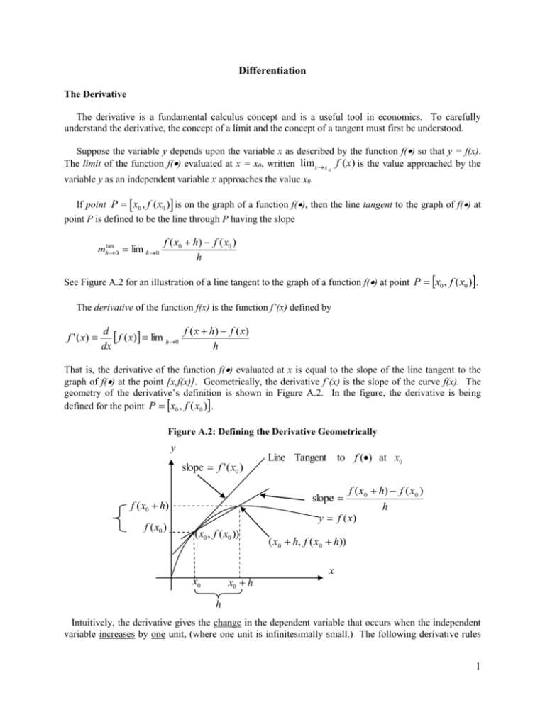
Differentiation
The Derivative
The derivative is a fundamental calculus concept and is a useful tool in economics. To carefully
understand the derivative, the concept of a limit and the concept of a tangent must first be understood.
Suppose the variable y depends upon the variable x as described by the function f() so that y = f(x).
The limit of the function f() evaluated at x = x0, written limx  x f ( x ) is the value approached by the
0
variable y as an independent variable x approaches the value x0.
If point P   x0 , f ( x0 ) is on the graph of a function f(), then the line tangent to the graph of f() at
point P is defined to be the line through P having the slope
mhtan0  lim h 0
f ( x0  h)  f ( x0 )
h
See Figure A.2 for an illustration of a line tangent to the graph of a function f() at point P  x0 , f ( x0 ).
The derivative of the function f(x) is the function f’(x) defined by
f ' ( x) 
d
 f ( x)  lim h0 f ( x  h)  f ( x)
dx
h
That is, the derivative of the function f() evaluated at x is equal to the slope of the line tangent to the
graph of f() at the point [x,f(x)]. Geometrically, the derivative f’(x) is the slope of the curve f(x). The
geometry of the derivative’s definition is shown in Figure A.2. In the figure, the derivative is being
defined for the point P  x0 , f ( x0 ).
Figure A.2: Defining the Derivative Geometrically
y
slope  f ' ( x0 )
f ( x0  h)  f ( x0 )
h
y  f (x)
slope 
f ( x0  h)
f ( x0 )
Line Tangent to f () at x0
( x0 , f ( x0 ))
x0  h
x0
( x0  h, f ( x0  h))
x
h
Intuitively, the derivative gives the change in the dependent variable that occurs when the independent
variable increases by one unit, (where one unit is infinitesimally small.) The following derivative rules
1
are useful in obtaining derivatives. The rules are given under the assumption that y is a dependent
variable, x is an independent variable, and c is a constant.
Constant Rule: If y = c then
dy
d

 c  0 .
dx dx
For example, if y = 5, then
dy
d

5  0 .
dx dx
Power Rule: y = xc then
 
dy
d c

x  cx c 1 .
dx dx
For example, if y = x5 , then
 
dy
d 5

x  5x 4
dx dx
A special case in which the power rule is used is when y = x. In
this case,
 
dy
d 1

x  1x 0  1
dx dx
Constant Coefficient Rule: If y = cf(x), then
dy
d
d
  cf ( x )  c  f ( x )  cf ' ( x )
dx dx
dx
For example, if y = 5x then
dy
d
d

5x )  5  x  5[1]  5

dx dx
dx
Sum Rule: If y = f(x) + g(x) then
dy
d
d
d
  f ( x )  g ( x )   f ( x )   g ( x ) 
dx dx
dx
dx
For example, if y = 5x + 2x2 , then


 
dy d
d
d

5 x  2 x 2  5 x  
2x 2  5  4x
dx dx
dx
dx
2
Product Rule: If y = f(x)g(x), then
dy
d
d
d
  f ( x ) g ( x )   g ( x )  f ( x )  f ( x )  g ( x )  g ( x ) f ' ( x )  f ( x ) g ' ( x )
dx dx
dx
dx
For example, if y = [5x][2x], then
dy
d
d
d
 [5x ][2x ]  2x 5x  5x  2x  2x[5]  5x[2]  10x  10x  20x
dx dx
dx
dx
Natural Log Rule: If y =ln(x), then
dy
d
ln ( x))  1

dx dx
x
For example, if y=5[ln(x)], then
dy d
d
1 5
 5ln ( x))   5 ln ( x))   5  
dx dx
dx
x x
Chain Rule: If y = f(g(x)), then
dy
d
d
d
  f ( g ( x )) 
f ( g ( x ))  g ( x )  f ' ( g ( x )) g ' ( x )

dx dx
d[g ( x )]
dx
For example, if y = (3+4x)2 then




dy d
d
d
3  4 x  2(3  4 x)(4)  8(3  4 x)  24  32 x

[3  4 x]2 
[3  4 x]2
dx dx
d [3  4 x]
dx
In economics, a given dependent variable typically depends upon more than just one independent
variable. For example, rather than a variable y merely depending upon a single variable x, the variable y
may depend upon three variables x1, x2, and x3 so that y = f(x1,x2,x3.). To find out how a change in one of
the independent variables affects the dependent variable, partial differentiation can be used. The partial
derivative y/x1 gives the change in the dependent variable y that occurs when the independent variable
x1 increases by one unit, assuming that the other independent variables x2 and x3 are constant.
Knowing which variables are to be treated as constant and which are allowed to vary, partial derivatives
can be calculated using the rules of differentiation described above. For example, suppose that
y  f (x1 , x2 , x3 )  3x1  x1x2  x32
To find out how the variable x1 affects y, take the derivative treating x1 as a variable, x2 as a constant, and
x3 as a constant:
3
y


3x1  x1x2  x32
x1 x1





3x1  
x1x2  
 x32 ,


x1
x1
x1



3x1  

 x1x2  ,
x1
x1


 3  x1   x2
 x1  ,
x1
x1
 

 3  x2
Sum Rule
Constant Rule
Constant Coefficient Rule
Power Rule
To find out how the variable x2 affects y, take the derivative treating x2 as a variable, x1 as a constant, and
x3 as a constant:
y


3x1  x1x2  x32
x2 x2





3x1  
x1x2  
 x32 ,


x2
x2
x2


 x1x2  ,
x2
 

 x1

 x2  ,
x2
Sum Rule
Constant Rule
Constant Coefficient Rule
 x1
Power Rule
Finally, to find out how the variable x3 affects y, take the derivative treating x3 as a variable, x1 as a
constant, and x2 as a constant:
y


3x1  x1x2  x32
x3 x3





3x1  
x1x2  
 x32 ,


x3
x3
x3


 x32 ,
x3
 

 

 2
x3 ,
x3
 2 x3
 
Sum Rule
Constant Rule
Constant Coefficient Rule
Power Rule
4
Implicit Differentiation
Consider the equation x1 x2  4 . Here, we can think of x1 as a function of x 2 , or we can think
of x 2 as a function of x1 . If we choose the latter, we could solve for x 2 and obtain the explicit
function x2  4 / x1 . That is, x2  f ( x1 ) , where f ( x1 )  4 / x1 is the function. The derivative
f ' ( x1 ) can then be found as f ' ( x1 )  dx2 / dx1  d[4 / x1 ] / dx1  4d[ x11 ]  4 x12  4 / x12 .
An alternative way of finding this derivative is to use implicit differentiation. Implicit
differentiation. Implicit differentiation is based upon the notion of the implicit function. When
we write x2  4 / x1 , we are emphasizing the we are thinking of x 2 as depending upon x1 (i.e.,
x 2 is a function of x1 ). However, when we write x1 x2  4 , we can still say x 2 is a function of
x1 . When we say this, we are recognizing a functional relationship that is implicit, but not
explicit. To implicitly differentiate the condition x1 x2  4 , we differentiate each side of the
equation first, and then solve for dx2 / dx1 .
To illustrate, we implicitly differentiate the equation x1 x2  4 by first writing
x1
d
x2   x2 d x1   d 4.
dx1
dx1
dx1
We have applied the product rule of differentiation here because in the condition x1 x2  4 , x1 is
obviously a function of x1 , and we are assuming x 2 is a function of x1 . These two functions of
x1 are in a multiplicative relationship, so we must apply the product rule. The next step is to
apply the differentiation rules and obtain.
x1
dx2
 x2  0 .
dx1
Finally, we need to solve for dx2 / dx1 . Doing so, we obtain
dx 2
  x 2 / x1 .
dx1
Because x2  4 / x1 , we can eliminate x 2 from this last expression and obtain dx2 / dx1  4 / x12 ,
which is the same result we obtained from directly differentiating the explicit function.
Differentials
The symbols dy and dx in the derivative dy / dx are called differentials. The symbol dy can
be interpreted as the change in the variable y that occurs as the variable x changes by dx .
Because the derivative is the slope of the line tangent to the function at the point in question,
5
these changes approximate the movement along the function y  f (x) . This approximation is
perfect when the function is linear. When the function is nonlinear, the change in y (i.e., dy )
becomes less accurate as the change in x (i.e., dx ) becomes larger.
The point here is that we can find derivates we are interest in by first taking differentials. The
rules for finding differentials are analogous to those for finding derivatives.
Constant Rule: If y = c then
dy  d [c]  0 .
For example, if y = 5, then
dy  d [5]  0 .
Power Rule: y = xc then
 
dy  d x c  cx c 1dx .
For example, if y = x5 , then
 
dy  d x 5  5x 4 dx
Constant Coefficient Rule: If y = cf(x), then
dy  d cf ( x)  cd  f ( x)  cf ' ( x)dx
For example, if y = 5x then
dy  d 5x  5d x  5[1]dx  5dx
Sum Rule: If y = f(x) + g(x) then
dy  d  f ( x)  g ( x)  d  f ( x)  d g ( x)
For example, if y = 5x + 2x2 , then


 
dy  d 5x  2 x 2  d 5x  d 2 x 2  5dx  4 xdx
Product Rule: If y = f(x)g(x), then
dy  d  f ( x) g ( x)  g ( x)d  f ( x)  f ( x)d g ( x)  g ( x) f ' ( x)dx  f ( x) g ' ( x)dx
For example, if y = [5x][2x], then
dy  d [5x][2x]  2xd5x  5xd2x  2x[5]dx  5x[2]dx  10xdx  10xdx  20xdx
6
Natural Log Rule: If y =ln(x), then
dy  d ln ( x))  
1
dx
x
For example, if y=5[ln(x)], then
5
1
dy  d 5ln ( x))   5d ln ( x))   5  dx  dx
x
x
Total Differentiation
Conceptually, total differentiation involves letting all variables in an equation change.
Reconsider the equation x1 x2  4 . If x1 changes, then x 2 must change in order for the equation
to still hold. If x1 and x 2 each change, then we must use the product rule. The differentiation
would be as follows.
d[ x1 x2 ]  d[4]
x1d[ x2 ]  x2 d[ x1 ]  0
x1dx2  x2 dx1  0 .
This last condition is the total differential of the equation x1 x2  4 . Notice, we can use this
condition to obtain the result dx2 / dx1  4 / x12 , which is what we obtained before.
Total differentials are especially useful when you want to find how one variable is affected by
more than one other variable in an implicit relationship. For example, consider the condition
f ( x  y )  g ( y  z ) . Notice that we cannot solve for the variable z in this condition. However,
let’s assume this equation implicitly defines z as a function of the variables x and y . We can
implicitly differentiate this condition as follows:
d [ f ( x  y )]  d [ g ( y  z )]
f ' ( x  y )d [( x  y ]  g ' ( y  z )d [( y  z )]
Chain rule
f ' ( x  y )[ dx  dy ]  g ' ( y  z )[ dy  dz ]
Constant coefficient rule
f ' ( x  y )dx  f ' ( x  y )dy  g ' ( y  z )dy  g ' ( y  z )dz
Algebra
dz  

f ' ( x  y)
f ' ( x  y) 
dx  1 
 dy
g ' ( y  z)
 g ' ( y  z) 
Algebra
7
This last condition is the total differential. We can obtain the partial derivative z / y by setting
dx  0 . That is,
z 
f ' ( x  y) 
.
 1 
y  g ' ( y  z ) 
This partial derivative tells us how z changes when x is held fixed (but y changes).
Similarly, the partial derivative
z
f ' ( x  y)

dx
x
g ' ( y  z)
tells us how z changes when y is held fixed (but x changes).
8