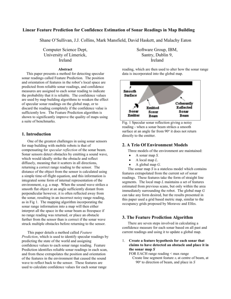
Linear Feature Prediction for Confidence Estimation of Sonar Readings in Map Building
Shane O’Sullivan, J.J. Collins, Mark Mansfield, David Haskett, and Malachy Eaton
Computer Science Dept,
University of Limerick,
Ireland
Abstract
This paper presents a method for detecting specular
sonar readings called Feature Prediction. The position
and orientation of features in the robot’s local space are
predicted from reliable sonar readings, and confidence
measures are assigned to each sonar reading to indicate
the probability that it is reliable. The confidence values
are used by map building algorithms to weaken the effect
of specular sonar readings on the global map, or to
discard the reading completely if the confidence value is
sufficiently low. The Feature Prediction algorithm is
shown to significantly improve the quality of maps using
a suite of benchmarks.
1. Introduction
One of the greatest challenges in using sonar sensors
for map building with mobile robots is that of
compensating for specular reflection of the sonar beam.
Sonar sensors detect obstacles by emitting a sound wave,
which would ideally strike the obstacle and reflect
diffusely, meaning that it scatters in all directions,
returning a correct range reading to the sensor. The
distance of the object from the sensor is calculated using
a simple time-of-flight equation, and this information is
integrated some form of internal representation of the
environment, e.g. a map. When the sound wave strikes a
smooth flat object at an angle sufficiently distant from
perpendicular however, it is often reflected away from
the sonar, resulting in an incorrect noisy range reading,
as in Fig 1. The mapping algorithm incorporating the
sonar range information into a map will then either
interpret all the space in the sonar beam as freespace if
no range reading was returned, or place an obstacle
further from the sensor than is correct if the sonar wave
struck multiple obstacles before returning to the sensor.
This paper details a method called Feature
Prediction, which is used to identify specular readings by
predicting the state of the world and assigning
confidence values to each sonar range reading. Feature
Prediction identifies reliable sonar readings in each scan,
and from these extrapolates the position and orientation
of the features in the environment that caused the sound
wave to reflect back to the sensor. These features are
used to calculate confidence values for each sonar range
Software Group, IBM,
Santry, Dublin 9,
Ireland
reading, which are then used to alter how the sonar range
data is incorporated into the global map.
Fig. 1 Specular sonar reflection giving a noisy
reading - when a sonar beam strikes a smooth
surface at an angle far from 90 o it does not return
directly to the emitter.
2. A Trio Of Environment Models
Three models of the environment are maintained:
 A sonar map S.
 A local map L.
 A global map G.
The sonar map S is a stateless model which contains
features extrapolated from the current set of sonar
readings. These features take the form of straight line
segments. The local map L maintains a set of features
estimated from previous scans, but only within the area
immediately surrounding the robot. The global map G
can take any form desired, but the results presented in
this paper used a grid based metric map, similar to the
occupancy grids proposed by Moravec and Elfes.
3. The Feature Prediction Algorithm
There are seven steps involved in calculating a
confidence measure for each sonar based on all past and
current readings and using it to update a global map.
1.
Create a feature hypothesis for each sonar that
claims to have detected an obstacle and place it in
the sonar map S
FOR EACH range reading < max range
Create line segment feature si at centre of beam, at
90o to direction of beam, and place in S
2.
3.
Compare each feature in S, si, with all the other
features in S, sj, to determine if they represent the
same object in the environment.
FOR EACH si in S
FOR EACH sj in S NOT EQUAL TO si
IF similar(si , sj) THEN
Create new feature sk between si and sj and
place it in S
Remove si and sj from S
Remove any feature in S caused by incorrect
readings. Confidence values derived from the
5.
Remove si from S and remove lj from L
FOR EACH si in S
Place si in L as a new segment
Remove si from S
Features in L too far from the robot are removed
FOR EACH li in L
IF dist(robot_position, last_position_detected(li))
> Td THEN
Remove li from L
6.
Generate final sonar confidence values, c da . For
any segment in L that should have been detected
but was not, split in two and shorten it.
Confidence values derived from the local model L
are denoted with a superscript L, with the
formula used to calculate the confidence value
s
sonar view are denominated by c x , where the s
signifies that this confidence value was derived
from the sonar view, and x indicates the formula
used to calculate it. An L superscript signifies that
the confidence value was derived from the local
map L.  is the difference in angle between the
sonar and the feature, and  is the beam
aperture.
FOR EACH sonj in SONARS
L
referred to with a subscript, as in c x .
FOR EACH soni in SONARS
c aL  c dL  0.5
FOR EACH lj in L
IF inconsistent(si , sonj) THEN
IF soni should sense lj if it exists THEN
c as  c ds  c aL  c dL  0.5
FOR EACH si in S
IF inconsistent(si , sonj) THEN
IF sonj should detect si THEN
   90    
c aL  0.5  
 * 0.25



   90    
c as  0.5  
 * 0.25



Divide lj at point of intersection with sonj,
creating lk and ll
Remove lj from L and insert lk and ll into L
Reduce length of lk and ll
IF length( lk ) < TL
Remove lk from L
IF length( ll ) < TL
Remove ll from L
IF soni should not sense lj if it exists THEN
ELSE IF sonj should not detect si
cds   R 2
2

s
c da
 combine c as , c as

FOR EACH li in L
IF inconsistent(li , sonj) THEN
IF sonj should detect li THEN
   90    
c aL  0.5  
 * 0.25



ELSE IF sonj should not detect li
cdL   R 2
2

L
c da
 combine c aL , c aL

FOR EACH si in S
IF si detected by only 1 sonar AND
( c da  Ts OR c da  Ts ) THEN
s
4.
L
Remove si from S
Compare all remaining features in S with all lines
in L, refining the hypothesis of the angle and
position of the features in L
FOR EACH si in S
FOR EACH lj in L
IF similar(si , lj) THEN
Create new feature between si and lj and place
it in L
L
cdL   R 2
2

L
c da
 combine c aL , c aL
7.

Use sonar confidence values to alter how the
sonar information is integrated into the global
map. The implementation of this step is specific
to the method being used to generate the global
map.
4. Calculating Confidence Values
A sonar beam is represented as three lines, as in Fig 4. If
none of the three lines intersect with a feature, then that
sonar is given a confidence value c da  0.5 , where X is
X
either s or L. The value 0.5 is used due to the fact that
when it is used in a Bayesian update formula, it has no
effect. If any of the three lines intersects with a feature
either in S or L then the sonar is inconsistent with that
X
X
feature. At this point, either c d or c a must be
calculated. If the difference in orientation between the
sonar and the feature is less than 25o (given a beam
aperture  of 25o), then the sonar should detect the
feature if the feature were at the predicted position and
orientation. In this case, the closer to perpendicular the
sonar is to the feature, the more likely it is to detect it.
As stated earlier, the initial confidence value of each
sonar is 0.5.
X
Therefore the confidence with regard to angle, c a , is
calculated as:
   90    
c aX  0.5  
 * 0.25



This maps the confidence value into the range [0.25,
0.5], meaning that a feature which should have been
detected by the sonar can, at worst, halve the confidence
in the sonar.
If the difference in orientation between the sonar beam
and the feature it is inconsistent with is more than 25 o
from perpendicular, then the sonar would not be
expected to detect the feature, assuming that it is a
smooth obstacle. In this case the confidence in the sonar,
Fig. 4. The predicted features in the sonar model S after
Step 1. The robot is facing straight into a wall with
sonars 2, 3, 4 and 5 returning a reading that is less than
the maximum range. Sonars 0, 1 and 6 return no
reading, and sonar 5’s reading, while less than the
maximum, is incorrect. The min/max possible angles
the line segments is in the [ ] brackets beside each line.
c dX is directly proportional to the distance from the sonar
to the feature.
cdX   R 2
2
When a range reading is inconsistent with a feature, only
the are behind the feature is updated incorrectly as being
freespace. The closer the feature is to the sonar, the
lower the confidence value must be to prevent the cells
behind the feature being effected by the map building
algorithm, as can be seen in Fig 2 and Fig 3.
Fig. 2. Sonar beam with an
undetected feature at
distance 1 from the
emitter. The darker the
area, the more strongly it is
believed to be unoccupied.
Fig. 3. Sonar beam with
undetected obstacle 2
from the emitter. The
strength of the freespace
update has been reduced.
Fig. 5. Predicted features after Step 2 is applied to the
sonar view from Fig 4. The three line segments S1 S2
and S3 have been merged to create one segment as their
min/max ranges overlap, and they are sufficiently close.
5. Combining Confidence Values
s
s
Once c d and c a have been computed, they are
combined to give a single confidence value for the sonar,
s
c da
. The confidence combination formulae are derived
from techniques for parallel combination of rules in
expert systems [1], with the full derivation available in
[2].
 2 cds cas
when cds  0.5 and cas  0.5
s
cda
 s
s
s
s
cd  ca  0.5 when cd  0.5 or ca  0.5
Fig. 6. State of the sonar model S after Step 3 has been
applied. Sonar 5 is inconsistent with the line created by
sonars 2, 3 and 4, and its confidence is low enough so
that the line predicted by it has been removed.

6. Experimentation Results
A suite of benchmarking techniques published in [3]
have been applied to 128 maps generated with and
without feature prediction, both in simulation and in real
world experiments on a Pioneer 1 robot from ActivMedia
robots. Each of the maps generated in the course of
experimentation are compared against hand drawn ideal
maps of the environment the robot traversed. A
complete description of all environments, benchmarks,
and procedures followed can be obtained from [2].
The four tests are as follows:
1. Correlation. A technique from the image
recognition field that tests the similarity of two maps
using the average and standard deviation the cells, as
well as comparing the maps on a cell-to-cell basis.
A higher percentage indicates a greater degree of
similarity between the maps.[4]
2. Map Score. A technique developed by Martin and
Moravec [5] which calculates the difference between
two maps by summing the squared difference of
corresponding cells in each map. The lower the
percentage difference, the greater the similarity
between the two maps.
3. Map Score of Occupied Cells. Similar to the
previous benchmark, but only tests those cells that
are occupied, i.e. >0.5 in one or both of the maps
being tested.
4. Path Comparison For False Positive Paths.
Examines the freespace areas of a map by
calculating the percentage of paths in the map which
would cause a robot to collide with an obstacle. The
lower the percentage, the fewer paths would cause a
collision, and therefore the better the map.
Correlation Map Map Score Path Comparison
Score Occupied False Positives
Cells
Without 59.77%
13.80% 11.05%
59.60%
Feature
Prediction
With
71.56%
9.18% 7.80%
40.20%
Feature
Prediction
6.1 Analysis of Results
All four benchmarks show considerable improvement
in map quality when Feature Prediction is applied.
 The correlation benchmark shows the map
quality increasing by 120%.
 The Map Score benchmark shows the map
quality increasing by 150%.
 The Map Score of Occupied Cells shows an
increase in map quality of 142%.
The Path Comparison for False Positive Paths
benchmark shows an increase of 148%.
7. Discussion
This paper presented a method of detecting specular
sonar reflections and assigning confidence values to the
sonar range readings in order to enable more accurate
map building. Experiments which employed the Feature
Prediction algorithm with a simple two-dimensional
gaussian sonar model from [6] showed an average
increase of map quality of 140% over four different
benchmarks. Performing Feature Prediction requires a
negligible amount of computational resources, with a
standard desktop workstation capable of performing
mapping for ten or more robots simultaneously.
However it vastly increases the quality of a map,
resulting in more effective navigation routines.
References
1. Heckerman, D. 1986. “Probabilistic interpretation
2.
3.
4.
5.
6.
for MYCIN's uncertainty factors.” Uncertainty in
Artificial Intelligence. L. N. L. Kanal, J.F. NorthHolland: 197-196.
O’Sullivan, S. 2003. An Empirical Evaluation Of
Map Building Methodologies in Mobile Robotics
Using The Feature Prediction Sonar Noise Filter
And Metric Grid Map Benchmarking Suite. MSc
Thesis, University of Limerick, Ireland.
Collins, J. J., O’Sullivan, S., Mansfield, M., Eaton,
M., Haskett, D. 2004. “Developing an extensible
benchmarking framework for map building
paradigms.”. In Proceedings Ninth International
Symposium on Artificial Life and Robots, Oita,
Japan, January 2004.
Baron, R. J. 1981. "Mechanisms of human facial
recognition." International Journal of Man Machine
Studies 15: 137-178.
Martin, M. C., Moravec, H.P. 1996. “Robot
Evidence Grids.” Robotics Institute, Carnegie
Mellon University, Pittsburgh, Pennsylvania
Moravec, H. P., Elfes, A. 1985. “High Resolution
Maps from Wide Angle Sonar.” Proceedings of the
1985 IEEE International Conference on Robotics
and Automation.