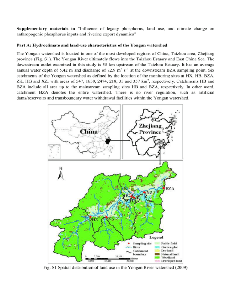
Supplementary materials to “Influence of legacy phosphorus, land use, and climate change on
anthropogenic phosphorus inputs and riverine export dynamics”
Part A: Hydroclimate and land-use characteristics of the Yongan watershed
The Yongan watershed is located in one of the most developed regions of China, Taizhou area, Zhejiang
province (Fig. S1). The Yongan River ultimately flows into the Taizhou Estuary and East China Sea. The
downstream outlet examined in this study is 55 km upstream of the Taizhou Estuary. It has an average
annual water depth of 5.42 m and discharge of 72.9 m3 s–1 at the downstream BZA sampling point. Six
catchments of the Yongan watershed as defined by the location of the monitoring sites at HX, HB, BZA,
ZK, HG and XZ, with areas of 547, 1650, 2474, 218, 35 and 357 km2, respectively. Catchments HB and
BZA include all area up to the mainstream sampling sites HB and BZA, respectively. In other word,
catchment BZA denotes the entire watershed. There is no river regulation, such as artificial
dams/reservoirs and transboundary water withdrawal facilities within the Yongan watershed.
Fig. S1 Spatial distribution of land use in the Yongan River watershed (2009)
Agricultural land (i.e., the sum of paddy field, garden plot, and dry land) averaged ~12% of total
watershed area, with developed land (i.e., the sum of rural and urban residential, roads, mining and
industrial), woodland, and natural lands contributing ~3%, ~67%, and ~18%, respectively, Fig. S1). Rice,
wheat, corn, vegetables, soybean, and potato are major crops cultivated in the agricultural lands. Due to
increased development, the areas of woodland and natural lands were decreased, while developed land
area was increased over the past 31 years, especially in the 2000s.
The climate of the Yongan watershed is subtropical monsoon with the six catchments having a long-term
average annual precipitation of 1308–1463 mm during 1980–2010 (Fig. S2). The rainfall mainly occurs in
May−September with the typhoon season usually occurring in July−September (Fig. S3). The Yongan
watershed has experienced some of the most significant regional climate change in Zhejiang Province
(The People’s Government of Zhejiang Province 2010). There has been a ~23 to ~28 day decrease in the
number of rainy days, and a ~65% to ~76% increase in the number of storm events (>50 mm per 24 hr)
over the 1980–2010 period. However, there were no significant trends in annual precipitation and average
river discharge over the study period (1980−2010) (Fig. S2). The long-term trends in these hydroclimate
variables were directly determined by regression analysis between each parameter and year number.
Daily precipitation data for the study period were obtained from three weather monitoring stations within
the Yongan watershed maintained by the Taizhou City Weather Bureau. Precipitation for each catchment
was calculated using the Thiessen polygon method to spatially distribute the single point record from rain
gauges, and the average precipitation was calculated by the following formula (Richard 1963):
P
A1
A
A
P1  2 P2    n Pn
A
A
A
(S1)
where, P is the mean rainfall of the region whose area is A, and P1, P2,…, Pn indicate rainfall samplings
within those polygons having areas A1, A2, …，An.
S1
6
150
100
2000
R2 = 0.1553, p<0.05
Precipitation
Discharge
R² = 0.000
a
0
9
HB
3
0
120
80
1500
40
R2 = 0.0350
1000
250
Rainy day
b
Storm number
R2 = 0.1424, p<0.05
200
HB
6
150
100
2500
2000
R2 = 0.1747, p<0.05
Precipitation
Discharge
a
0
9
BZA
R² = 0.000
3
0
150
110
70
1500
R² = 0.023
1000
250
Rainy day
b
Storm number
R2 = 0.1955, p<0.05
200
150
100
2800
BZA
6
R2 = 0.1587, p<0.05
a
Precipitation
Discharge
R² = 0.000
2200
30
9
ZK
3
0
15
10
5
1600
1000
250
R² = 0.071
Storm number
R2 = 0.1311, p<0.05
b
Rainy day
a
R2 = 0.1954, p<0.05
Precipitation
Discharge
200
ZK
150
0
12
8
4
100
2500
2000
HG
R² = 0.000
2
R² = 0.023
1
0
9
1500
Rainy day
b
Storm number
R2 = 0.1264, p<0.05
HG
6
150
100
2500
2000
R2 = 0.1587, p<0.05
a
Precipitation
Discharge
XZ
8
R² = 0.023
Rainy day
b
Storm number
R2 = 0.1264, p<0.05
200
150
100
1980
3
0
24
16
R² = 0.000
1500
1000
250
0
3
XZ
1984
1988
1992
1996
2000
2004
Discharge
(m3 s-1)
0
9
6
3
R2 = 0.1587, p<0.05
Storm
number
HX
Discharge
(m3 s-1)
200
Storm number
R2 = 0.1502, p<0.05
Storm
number
Rainy day
b
Discharge
(m3 s-1)
1000
250
Storm
number
12
R² = 0.017
Discharge
(m3 s-1)
24
1500
1000
250
200
36
Storm
number
HX
Discharge
(m3 s-1)
Discharge
R² = 0.000
Storm
number
Precipitation
Discharge
(m3 s-1)
a
Storm
number
Precipitation
(mm yr-1)
Precipitation Rainy day
(mm yr-1)
number
Precipitation Rainy day
(mm yr-1)
number
Precipitation Rainy day
(mm yr-1)
number
Precipitation Rainy day
(mm yr-1)
number
Precipitation Rainy day
(mm yr-1)
number
Rainy day
number
2000
0
2008 2010
Fig. S2 Changes of hydroclimate variables in each of the six catchments within the Yongan watershed
from 1980 to 2010: precipitation and river water discharge (a), annual number of rainy days and number
of storm events (b)
S2
Monthly precipitation (mm)
350
300
250
200
150
100
50
0
Jan. Feb. Mar. Apr. May. Jun. Jul. Aug. Sep. Oct. Nov. Dec.
Fig. S3 Average monthly precipitation in the Yongan watershed in 1980–2010. The error bars refer to
standard deviations of measurements from the three weather monitoring sites within the watershed
Part B: Riverine TP flux estimate
River water samples were collected once every 4–8 weeks during the 1980–2010 period at six monitoring
sites (Fig. S1). Water samples were collected between 8:00 and 9:00 and total phosphorus (TP) was
analyzed in the certified laboratory of the Taizhou City Environmental Protection Bureau. Well mixed
water samples (surface and bottom layers at three sites along the cross section) were collected and
composited. Duplicate water samples were collected from the composite for analysis. The water samples
were acidified with H2SO4 in the field (10 ml of concentrated H2SO4 per liter of sample) and analyzed
within 4 hr after sampling. TP concentration (all dissolved and particle phosphorus) in the unfiltered
water samples was determined by the spectrophotometric ammonium molybdate method (limit of
detection: LOD = 0.01 mg P L-1), recommended by The Ministry of Environmental Protection of the
People's Republic of China (State Environmental Protection Administration of China 2002). River
discharge was measured once every 2 to 12 hours using the rotating-element current-meters method
following the standard method recommended by The Ministry of Water Resources of the People's
Republic of China (The Ministry of Water Resources of the People's Republic of China 1995).
To estimate annual TP flux using the discrete monitoring data from 1980–2010, the widely applied
LOADEST model was utilized to predict daily TP flux (Runkel et al. 2004):
Ln( Lt )  0  1Ln(Qt )  2 Ln(Qt )2  3t  4tc  5 sin( 2t )  6 cos(2t )
2
(S2)
where Ln is the natural logarithm function; Qt is daily average river discharge for a given P monitoring
date (m3 s–1), Lt is the measured daily P flux (kg P d–1), which is estimated by multiplying measured P
concentration by Qt; t is the decimal time for the corresponding monitoring date; tc is the center of
decimal time for the study period (a constant); β0...β6 are the fitted parameters in the multiple regression;
β1 and β2 describe the relation between flux and discharge; β3 and β4 describe the relationship between
flux and time; and β5 and β6 describe seasonal variation in flux data.
In this study, the LOADEST model parameters shown in Eq. S2 (i.e., β0...β6) were calibrated by least
squares fit using Matlab software (version 10.0, The MathWorks, Inc., US, 2010) for each of the six
catchments. All calibrated parameter values were statistically significant (p<0.05) with average relative
errors of ±4%–±15% and high R2 between the modeled and measured TP concentration (Table S1). These
S3
results indicate that the established LOADEST models can be reasonably applied to estimate daily TP
concentrations in the Yongan watershed (Fig. S4). Here, daily TP load was estimated by multiplying TP
concentration and water discharge, and annual TP load was calculated from the sum of daily TP loads for
a corresponding year. Annual TP flux was determined by dividing the annual TP load by the total drainage
area upstream of each monitoring station.
Table S1 The calibrated LOADEST parameters for TP concentration for each of the six catchments in the
Yongan watershed
Catchm Parame
β0
β1
β2
β3
β4
β5
β6
R2
ent
ter
Mean
-8.838
-0.119
0.015
0.282
0.179
4.501
-0.161
0.76
HX
-12.842
-0.273
-0.068
0.026
-0.062
2.449
-0.235
(n=176)
95% CI
-5.835
0.036
0.097
0.539
0.420
6.553
-0.086
Mean
-4.079
0.008
0.015
-0.007
0.169
0.057
0.001
0.98
HB
-4.475
-0.085
-0.034
-0.191
-0.024
0.046
-0.001
(n=174)
95% CI
-3.683
0.100
0.064
0.178
0.362
0.067
0.003
Mean
-3.094
-0.117
-0.032
-0.199
-0.012
0.094
-0.0004
0.78
BZA
-4.165
-0.171
-0.059
-0.293
-0.108
-0.104
-0.009
(n=183)
95% CI
-2.023
-0.062
-0.004
-0.105
0.087
0.292
0.008
Mean
-5.458
-0.098
-0.016
-0.057
-0.0211
0.0100
-0.002
0.92
ZK
-8.275
-0.205
-0.069
-0.198
-0.160
-0.348
-0.019
(n=174)
95% CI
-2.640
0.010
0.038
0.084
0.118
0.547
0.016
Mean
-5.457
-0.201
-0.003
0.038
0.247
0.732
-0.033
0.87
HG
-16.440
-0.370
-0.097
-0.296
-0.103
-0.971
-0.098
(n=170)
95% CI
5.527
-0.032
0.092
0.371
0.598
2.436
0.032
Mean
-4.912
-0.221
0.019
-0.513
0.239
0.227
-0.005
0.78
-9.848
-0.447
-0.096
-0.855
-0.088
-0.633
-0.041
XZ
(n=151)
95% CI
0.024
0.005
0.135
-0.171
0.566
1.086
0.031
S4
1000
100
10000
R2=0.72
n=176
1000
10
100
1
10
-1
Modeled TP load (kg P d )
0.1
0.01
0.01
10000
1000
1
10
HB
1
HX
0.1
R2=0.98
n=174
100 1000
R2=0.78
n=183
0.1
0.1
100
1
10
100 1000 10000
R2=0.92
n=174
10
100
1
10
1
0.1
0.1
1000
100
0.1
BZA
1
10
100
1000 10000
R2=0.87
n=170
0.01
0.01
1000
10
1
1
HG
0.1
0.1
1
10
1
0.1
10
0.1
100 1000
0.01
0.01
100
R2=0.78
n=151
100
10
0.001
0.01
ZK
XZ
0.1
1
10
100 1000
-1
Measured TP load (kg P d )
Fig. S4 Measured daily riverine TP load versus the modeled values using the LOADEST model for each
of the six catchment in the Yongan watershed
It is well known that nutrient inputs to rivers from point and nonpoint sources demonstrate significant
hydrological differences. Point source nutrient input to rivers is relatively constant and hydrologically
independent. In contrast, diffuse source nutrient inputs have a strong hydrologic dependence (Chen et al.
2013; Bowes et al. 2014). To address the role of point and nonpoint source P input to rivers, relationships
between measured riverine TP concentration and water discharge in the six catchments were evaluated.
Among the six catchments of the Yongan watershed, catchment ZK demonstrated a significant positive
relationship between river TP concentrations and river discharge, while catchment HG presented a
significant negative correlation (Fig. S5). These results indicate that P inputs from nonpoint (erosion and
leaching) and point (domestic sewage) sources are the dominant cause of riverine TP in catchments ZK
and HG, respectively (Chen et al. 2013; Bowes et al. 2014). No significant correlations were observed in
the other four catchments, implying that P inputs from both point and nonpoint source produced
comparable contribution to riverine TP flux (Fig. S5).
S5
0.1
0.09
HB
HX
0.08
P >0.05
0.06
0.06
P >0.05
0.04
0.03
0.1
10
0.3
1000 0.1
BZA
0
1000
0.03
10
ZK
y = 0.0118x0.0395
0.2
2
R = 0.12, P <0.01
P >0.05
0.02
0.1
0.01
0
0.1
1.2
0.9
0.6
1
10
100
1000 0.01
HG
y = -0.0227Ln(x) + 0.2053
R2 = 0.11, P <0.01
0.1
1
10
100
0.3
XZ
0.2
P >0.05
0.1
0.3
0
0.01
-1
-1
TP concentration (mg L )
0
TP concentration (mg L )
0.02
0
0.1
1
10 0.1
1
10
3 -1
River water discharge (m s )
100
Fig. S5 The relationship between TP concentration and river discharge for each of the six catchments in
the Yongan watershed
Part C: Soil characteristics and management
There are 5 soil groups, including 10 soil subgroups and 130 soil species, in the Yongan watershed. The
red, yellow, and lithological soil groups were the dominant soil types and accounted for 64.6%, 15.4%,
and 1.5% of total soil area in the watershed, respectively (Agricultural Bureau of Xianju County 2011).
The dominant red and yellow soil groups correlate with Oxisols and Ultisols in USDA Soil Taxonomy.
The alluvial and paddy soil groups were the dominant soil types in the plain area and accounted for 3.9%
and 14.6% of total soil area, respectively. Extensive soil property measurements were conducted in 1984
and 2009 by the Agriculture Bureaus of Xianju County in Zhejiang Province, China (Soil Survey Office
of Taizhou City 1987; Agricultural Bureau of Xianju County 2011; Chen and Lu 2013). In 1984, soil
properties for the 0–20 cm, 20–40 cm, 40–100 cm soil layers of the different soil types and agricultural
land types were hierarchically measured, which was supported by the Second National Soil Census of
China. In 2009, soil samples were collected from the same locations as in 1984 and soil properties for the
upper 20-cm layer of the different soil and farmland types were measured, which was supported by the
S6
National Soil Measurement and Formulated Fertilization Program of China. On average, one composite
sample was collected per 15 ha for plain region soils and one sample per 25 ha for hilly region soils.
Composite soil samples (20–30 subsamples from each 15–25 ha area) were collected from the upper
20-cm soil layer in October to December following crop harvest. Undisturbed soil samples were
simultaneously collected in cylindrical cores for measuring soil bulk density. Soil samples were air-dried,
milled, and passed through a 2-mm sieve for chemical analysis. Soil total P (TP) content and Olsen P
were measured by the H2SO4-HClO4 degradation (all organic and inorganic P in soil sample were
transformed into PO4-P in the solution)-molybdenum antimony colorimetric method and NaHCO3
extraction-molybdenum antimony colorimetric method (Agricultural Chemistry Specialty Committee of
Soil Science Society Chinese 1983), respectively. Soil pH was measured potentiometrically using a pH
meter in a 1:5, soil:distilled water suspension. To be comparable, data measured in the same catchment
for upper 20-cm layer in both 1984 and 2009 (Table S2) were used to address the changes in soil
properties over the 25 year period between sample collections.
Table S2 Changes of soil properties in the upper 20-cm soil layer of agricultural lands in the Yongan
watershed between 1984 and 2009
1984
2009
Catchment
Bulk density
Olsen P
TP
Bulk density
Olsen P
TP
pH
pH
3
–1
–1
3
–1
(g cm )
(mg P kg ) (mg P kg )
(g cm )
(mg P kg ) (mg P kg–1)
1.12a
Mean 5.1a
10b
211b
5.3a
1.11b
49a
581a
HX 97.5% 6.1
1.34
100
611
6.4
1.35
341
1220
2.5% 4.2
0.87
2.0
71
4.5
0.76
9
212
1.2a
Mean 5.1a
11.1b
220b
5.1a
1.18a
41a
419a
HB 97.5% 6.2
1.54
185
586
6.3
1.46
312
843
2.5% 4.1
0.92
1.2
44
4.2
0.86
5.1
98
1.1a
1.15a
Mean 5.0a
15.9b
255b
5.1a
32a
490a
BZA 97.5% 6.4
1.3
117
870
6.3
1.24
453
1232
2.5% 4.2
0.77
1.0
43
4.1
0.8
7.2
109
1.21a
1.18a
Mean 4.8a
8.8b
144b
4.9a
56a
629a
ZK 97.5% 6.0
1.45
53
521
5.9
1.51
184
1132
2.5% 4.0
0.82
2.0
46
4.1
0.76
13
123
1.21b
1.15b
Mean 5.2b
15b
157b
5.4a
49a
443a
HG 97.5% 6.3
1.72
98
572
6.4
1.64
287
829
2.5% 4.5
0.91
1.2
26
4.7
0.89
2.2
110
1.31a
1.21a
Mean 5.5a
24.2b
241b
5.1b
57.2a
503a
XZ 97.5% 6.3
1.81
108
750
6.2
1.77
470
1321
2.5% 4.8
0.86
1.3
50
4.9
0.71
12
128
Lower case letters denote significant differences in soil properties between 1984 and 2009 in each
catchment (p<0.01).
Using the measured changes in soil TP content, cumulative P accumulation (S20cm, kg P ha–1) in the upper
20-cm layer of agricultural soils between 1984 and 2009 was estimated as follows:
S7
3
S20cm 
C
i 1
09,i
3
B09,i A09,i 10   C84,i B84,i A84,i 104
4
i 1
(S3)
Aw
where C84,i, B84,i, and A84,i are P content (mg P kg–1), soil bulk density (g cm–3), and area for ith land-use
type (ha) within the catchment in 1984; C09,i, B09,i, and A09,i are P content (mg N kg-1), soil bulk density (g
cm–3), and area for ith land-use type (ha) within the catchment in 2009; and Aw is catchment area (ha).
The majority of agricultural irrigation and drainage systems used in 1980−1999 time period was
constructed with stone and mud in the 1950s and progressively lost water delivery capacity after 20−30
years due to silting and collapse. Therefore, agricultural lands became waterlogged during the rainy
season (May−September), especially during the typhoon season (Fig. S3), resulting in a considerable crop
yield reduction. To cope with more frequent storm events (Fig. S2) and increasing water use conflicts
between agriculture and industry, local government investment was increased to renovate old irrigation
and drainage systems during the past 31 years. The agricultural land area irrigated and drained with old
channels decreased by 40−80% between 1980 and 1999 (Fig. S6). In 2000−2009, new cement channels
and pipes established in agricultural lands rapidly increased by 1.5-fold to 3.1-fold. Thus, the efficiency
of agricultural drainage conveyance (drained agricultural land area) was greatly improved. The data on
the agricultural areas drained by old and renovated drainage systems for each of 21 towns within the
Yongan watershed were derived from the annual Statistic Yearbook of Xianju County and Statistic
Yearbook of Linhai City.
S8
2000
HX
1000
20%
10%
500
0
6000
0%
40%
HB
Drained agricultural land area (ha)
4000
20%
2000
0
12000
9000
6000
3000
0
200
150
100
50
0
500
400
300
200
100
0
1500
0%
40%
BZA
20%
0%
20%
15%
10%
5%
0%
60%
ZK
HG
Drained area percentage
1500
30%
Old channel
Renovated channel
Drained area percentage
40%
20%
0%
30%
XZ
1000
20%
500
10%
0%
0
1980
1985
1990
1995
2000
2005
2010
Fig. S6 Changes of agricultural land area and percentage of agricultural lands drained with old and
renovated channels in the six catchments of the Yongan watershed in 1980−2010
Part D: NAPI calculation and uncertainty analysis
1. Data source
Data sources for estimating the annual NAPI budget for the six catchments of the Yongan watershed and
agricultural drainage system from 1980 to 2010 were derived from the annual Statistic Yearbook of
Xianju County and Statistic Yearbook of Linhai City. By defining the watershed boundary using a
geographical information system (GIS), all towns within Xianju County (~73% of total watershed area)
and one town in Linhai City (~12% of total watershed area) were included within the watershed boundary.
The remaining ~15% of the catchment area only considered the P input from atmospheric deposition in
the NAPI analysis, since it was dominated by forests (~95%) and fell within Panan County (located in the
northwest portion of the watershed) and Jinyun County (located in the southwest portion of the watershed)
S9
(Fig. S1).
2. NAPI estimation
NAPI was calculated as the sum of four major components: atmospheric P deposition, P fertilizer
application, non-food P, and net P in food, feed and seed import/export, where the net food, feed and seed
P input was calculated as the sum of human and livestock P consumption and seed input minus the sum of
P contained in livestock and crop production (Han et al. 2013). Pesticide P input was also a component
for NAPI, but it represented less than 0.001% compared with P fertilizer according to the records in the
Statistic Yearbooks; thus, pesticide P input was neglected in this study. NAPI for each of 21 towns within
the watershed was estimated for addressing the spatial distribution. Based on the defined boundary for
each catchment using GIS, NAPI for a town that belongs to two or more catchments was allocated among
catchments using the land-use area ratio method (Han et al. 2011). To match estimated catchment NAPI
with riverine TP fluxes at the six sampling sites (Fig. S1), the catchments HB and BZA include all
watershed area up to the mainstream sampling sites HB and BZA, respectively (Table 1).
2.1 Fertilizer P application
Annual commercial chemical and organic P fertilizer input was estimated from the applied amount of
each fertilizer type and corresponding P content. Annual phosphorus fertilizer application amounts, such
as superphosphate, calcium-magnesium phosphate, monoammonium phosphate and diammonium
phosphate, in 1980−2010 were directly collected from the statistical yearbooks. P fertilizer contained
12−18% of P2O5 (Liang 1999). Total P fertilizer application was converted to kg P by multiplying by
436.4 kg P per ton P2O5 (Han et al. 2013).
2.2 Atmospheric P deposition
Atmospheric P deposition rate considered both wet and dry deposition. Wet P deposition was estimated
by multiplying TP concentration in rainwater and annual precipitation. Considering <3.5% of the urban
area percentage and >65% of the forest area in the Yongan watershed, it can be considered in the Class VI
category with TP concentration in rainwater of 0.005 mg L-1 according to the reviewed results concerning
TP concentration in precipitation by Zhang and Jøgensen (2005) and Wu and Chen (2013). Then annual
wet P deposition was estimated from the product of TP concentration and annual precipitation. The dry P
deposition was estimated from the ratios between dry and wet deposition rate observed in the nearby
Taihu Lake area (Liu et al. 2012), i.e., 60%, 252% and 299% in 1987−1988, 2002−2003 and 2010,
respectively. Linear interpolation was adopted to estimate annual dry P deposition rates between reported
values. Finally, atmospheric P deposition for the six catchments was estimated as the sum of wet and dry
P deposition rates, which varied from 0.09 to 0.39 kg P ha–1 yr–1 from 1980 to 2010. These estimated
results were consistent with previous observations conducted for Eastern Asia over the 1954−2012 period
(0.075−1.1 kg P ha–1 yr–1, Tipping et al. 2014) and for the Taihu Lake watershed over the 1987−2011
period (0.024−0.35 kg P ha–1 yr–1, Liu et al. 2012).
2.3 Seed P input
In this study, we took seed P as an input for NAPI estimates. Vegetables and the six main agricultural
crops, which are major agricultural plants in the watershed, were considered for estimating seed P input.
Seed P per unit area for each crop type was adopted from the results of Han et al. (2013) and Wang et al.
(2009) as shown in Table S3. Seed P input was then estimated by multiplying the seed P input per unit
area for each crop type by the cultivated area of the watershed.
Table S3 Seed P input rate per unit area for each crop type
S10
Crop type
Rice
Wheat
Corn
Potato
Soybeans
Peanuts
Vegetables
Seed P (kg P km–2 yr–1)
6.43
23.81
4.53
79
8.90
0.58
0.03
2.4 Non-food P
Non-food P input was largely derived from detergent used in people’s daily lives. Inputs were estimated
by multiplying the annual detergent consumption per person by P content in detergent and by the
population of each catchment. From 1980 to 2010, the annual detergent consumption per person was
increased year by year, with 0.40, 2.41, 2.50, 3.12, 4.12 and 6.16 kg person–1 yr–1 in 1980, 1996, 2000,
2001, 2005 and 2010, respectively (Shu et al. 1998; CCIA 2001; Jin et al. 2001; China Surfactant
Network 2007; He et al. 2009; China-Consulting Network 2011). Linear interpolation was adopted to
estimate annual detergent consumption for years in which data were not available. Though the
government put forward a “phosphorus forbidden” policy for Zhejiang Province in 2004, non-P detergent
for consumption is less than 10% of total use due to high production cost (Ji 2007a). Thus, P content in
detergent was considered as a constant of 4.25% (Ji 2007b).
2.5 P in net food and feed imports
Phosphorus in net food and feed imports was calculated as the sum of human P consumption and
livestock P consumption, minus the sum of P contained in livestock and crop production (Han et al. 2013).
Human consumption of P in food was estimated by multiplying the number of inhabitants (Fig. S7) by a P
intake rate per capita. The value of the per capita intake of phosphorus for each year was derived from
Han et al. (2013) and Sprague and Gronberg (2013), i.e., 0.39, 0.46, and 0.52 kg in 1980, 2002, and 2009,
respectively. We linearly interpolate values for missing years using the reported values.
Domestic animals in China are usually fed according to relatively straightforward dietary prescriptions
designed for maintaining or gaining weight. The P mass in animals was calculated as the P consumption
per individual animal multiplied by the number of each animal type. The values of P consumption per
individual animal were obtained from Han et al. (2013) (Table S4). Using Eq. S3, the average animal
population for a year was quantified using data on sales and inventory of livestock (Hong et al. 2013).
AL  inventory 
1
Sales Cycles  1


Cycles Cycles
Cycles
(S3)
where AL is the annual average number of livestock, inventory is the number population from the
end-of-year inventory data (Figure S7), Sales is the number of livestock slaughtered, which was derived
from the Statistics Yearbooks, and Cycles is the duration of the life cycle (the number of days from birth
to market) per year, which is estimated as: 365/life cycle. The life cycle for each animal type was adopted
from the results reported by Wang et al. (2006) for China. We assumed all animals were completely
formula fed, i.e., 80% from corn and 20% from pasture (Li 2007).
S11
0
1.2
30
0.8
15
0.4
Human
Cattle and Cow
Hog
Sheep and Goat
3
3
3
2010
2008
2004
2000
1996
1992
1988
1984
0
1980
0
0
120
0
12
XZ
80
8
40
4
0
0
1980
HG
0.5
Chicken and Duck
Rabbit
Sheep and goat, cattle and cow, rabbit populations (10 ), aquatic production (10 t)
0
45
20
2010
10
2008
200
1.0
2004
20
400
ZK
40
2000
600
0
1.5
0
60
1996
30
200
1992
BZA
800
10
1988
0
40
0
1000
400
1984
5
20
600
3
50
HB
800
Human, hog, chicken and duck populations (10 )
10
30
1000
3
100
3
Human, hog, chicken and duck populations (10 )
HX
Sheep and goat, cattle and cow, rabbit populations (10 ), aquatic production (10 t)
15
150
Aquatic product
Fig. S7 Annual population and end-of-year inventory for different types of livestock in each catchment
for the Yongan River watershed in 1980−2010
Livestock type
Pigs
Horses and cattle
Sheep
Chickens
Duck
Aquatic products
(kg P Mg–1)
Table S4 Livestock P consumption and excretion rates
P consumption (kg P
P excretion (kg P
–1
–1
individual yr )
individual–1 yr–1)
4.59
3.17
10.99
9.78
1.26
1.06
0.18
0.12
0.34
0.22
0.56
2.16
Production P (kg P
individual–1 yr–1)
1.42
1.21
0.2
0.06
0.12
1.60
Livestock P production was the difference between livestock P consumption and livestock P excretion.
The values for the percentage of P excreted were obtained from Han et al. (2013) (Table S4). It was
assumed that spoilage and inedible components caused a 10% loss of animal product available for
consumption (Han et al. 2013).
Crop P production was estimated by multiplying the yield of a specific crop (Fig. S8) by its P content.
S12
The P contents (g kg–1) for different crops are listed in Table S5. The P content in different fruits is only
slightly different such as apples, grapes, peaches and pears; thus we used the average data for these fruits
to represent all fruits (Han et al. 2013). We assume that pests, spoilage and processing cause a 10% loss
for all crops (Han et al. 2013).
2.4
40
24
160
HX
HB
30
120
200
10
5
100
0
75
0
0.12
HG
50
0.08
25
8
0
12
0
0.6
ZK
9
0.4
6
0.2
3
0
56
0
1.8
XZ
42
1.2
6
40
Soybean, peanut and corn yields (10 kg)
6
0
15
BZA
Soybean, peanut and corn yields (10 kg)
10
0
300
80
6
0.8
Rice, wheat, potato,fruits and vegetable yields (10 kg)
16
20
6
Rice, wheat, potato,fruits and vegetable yields (10 kg)
1.6
28
0.04
0.6
14
Rice
Corn
Wheat
Soybean
0
Potato
Peanut
Fruits
2010
2008
2004
2000
1996
1992
1988
0
1980
2010
2008
2004
2000
1996
1992
1988
1984
1980
0
1984
0
Vegetable
Fig. S8 Annual yields of major crops for the six catchments of the Yongan watershed in 1980−2010
Table S5 P content of agricultural crops
Crop type
P content (g kg–1)
Rice
1.10
Corn
2.44
Wheat
1.88
Potato
0.40
Peanuts
2.50
Soybeans
4.65
Vegetable
0.30
Fruits
0.13
2.6 Phosphorus weathering from soil parent material
The dominant soils in the Yongan River watershed are highly weathered red and yellow soils (~90% of
entire watershed area; Oxisols and Ultisols) that contribute a very limited background P flux compared to
NAPI sources (Zhang et al. 2005). This assumption is supported by a study in the Lake Dianchi watershed
in southern China where red soils were found to contribute 0.006 kg P ha–1 yr–1 via natural rock
S13
weathering (Liu 2005). Similarly, the low TP export coefficients observed in several natural ecosystems
indicate low weathering rates (0.0085 kg P ha–1 yr–1, USEPA 2002). As a result, the weathering P inputs
were not considered in this study. Additional studies are required to verify the contribution from natural
background P sources.
3. Uncertainty analysis in NAPI estimation
To gain insight into the uncertainty in the NAPI estimation, an uncertainty analysis was performed using
Monte Carlo simulation, which utilized random sampling from probability distribution functions as inputs
(Hendren et al. 2013). The Monte Carlo method assumes that the uncertainty of the model inputs can be
characterized by their statistical distribution functions; thus it is useful in modeling systems characterized
by uncertainty through giving a measure of uncertainty for calculated quantities. Due to the limited
information available for China and surrounding regions, we can not rigorously determine the probability
distribution and coefficient of variation for each parameter used in estimating NAPI. Therefore, we
assumed that all the parameters used in the NAPI estimation followed a normal distribution with a
coefficient of variation equal to 30% for each parameter, which is commonly used in nutrient budgeting
studies of nearby watersheds (Yan et al. 2011; Ti et al. 2012). All input parameters (Table S3−S5) for
estimating NAPI were set to be independent of each other during the Monte Carlo sampling, since the
majority of the parameters have no cause-and-effect relationship with each other in theory and the
dependence (correlation) is difficult to quantify due to the limited information. The Monte Carlo
sampling method was used to randomly generate 10,000 sets of model parameters according to their
normal distribution functions, resulting in 10,000 iterations of NAPI simulation for each year to obtain
the mean and 95% confidence interval for annual NAPI values. The NAPI estimation procedure was
formulated in Microsoft Excel 2007 embedded with Crystal Ball software (Professional Edition 2000,
Oracle Ltd. US., 2000) to run Monte Carlo simulations.
Part E: Regression models for riverine TP export
Table S6 Results of multiple regressions between annual riverine TP yield (F, kg P ha–1 year–1) and NAPI
(kg P ha–1 year–1), precipitation (P, mm year–1), number of storm events (SE), developed land area
percentage (D%), and drained agricultural land area percentage (DA%). All regressions were significant at
p<0.001.
Nash
Model formulas
R2
Sutcliffe
F  0.0081P1.752 exp( 0.430 NAPI )
0.78
0.77
F  0.0089SE 0.383 exp( 0.433NAPI )
0.77
0.75
F  0.464D%0.719 exp( 0.282 NAPI )
0.81
0.80
F  0.478DA%1.516 exp( 0.272 NAPI )
0.86
0.84
F  0.291P1.760DA%1.517 exp( 0.256 NAPI )
0.88
0.87
F  0.314 P1.891D%0.749 exp( 0.259 NAPI )
0.84
0.84
S14
F  0.356SE 0.481DA%1.602 exp( 0.247 NAPI )
0.89
0.88
F  0.500SE 0.540D%0.848 exp( 0.236 NAPI )
0.84
0.83
F  0.379 P1.779DA%1.404 D%0.109 exp( 0.245NAPI )
0.94
0.92
F  0.585SE 0.506DA%1.390 D%0.207 exp( 0.233NAPI )
0.89
0.88
F  0.468P0.975SE 0.349DA%1.382 D%0.189 exp( 0.225NAPI )
0.89
0.87
Reference
Agricultural Bureau of Xianju County (2011) Agricultural ecological environment quality assessment in
the Xianju County. http://www.xjlsncp.com/html/main/nyqhView/2011-12/6533.html. (in Chinese)
Bowes J, Jarviea HP, Naden PS, Old GH, Scarlett PM, Roberts C, Armstrong LK, Harman SA, Wickham
HD, Collins AL (2014) Identifying priorities for nutrient mitigation using river concentration–flow
relationships: The Thames basin, UK. J Hydrol 571:1–12. doi: 10.1016/j.jhydrol.2014.03.063
Chen DJ, Dahlgren RA, Lu J (2013) A modified load apportionment model for identifying point and
diffuse source nutrient inputs to rivers from stream monitoring data. J Hydrol 501:25–34. doi:
10.1016/j.jhydrol.2013.07.034
Chen HS, Lu LY (2013) Characteristics of soil fertility of farmlands in red earth area in Xianju County,
eastern Zhejiang Province. J Henan Agr Sci 42:65–67 (in Chinese)
Chen J, Wu XD, Brian LF, Webber M, Wei TY, Li MT, Chen ZY (2014) Variability and trend in the
hydrology of the Yangtze River, China: Annual precipitation and runoff. J Hydrol 513:403–412.
doi: 10.1016/j.jhydrol.2014.03.044
China Cleaning Industry Association (CCIA) (2001) Detergent with phosphorus is safe to human and
environment. Surfactant Soap and Detergent Industry of China 4:5–7 (in Chinese)
China Surfactant Network (2007) Industrial status of synthetic detergent and surfactant demand in China.
http://www.chinasurfactant.net/index.php/index/detail/id/3128 (in Chinese)
China-Consulting Network (2011) Depth analysis report about detergent industry in China, 2010.
http://www.china-consulting.cn/article/html/2011/1125/147241.php (in Chinese)
Chinese Agricultural Chemistry Specialty Committee of Soil Science Society (1983) Routine Analysis
Method of Soil Agricultural Chemistry. Chinese Science Press, Beijing (in Chinese)
Feng ZJ, Schilling KE, Chan KS (2013) Dynamic regression modeling of daily nitrate-nitrogen
concentrations in a large agricultural watershed. Environ Monit Assess 185:4605–4617. doi:
10.1007/s10661-012-2891-7
Han Y, Li X, Nan Z (2011a) Net anthropogenic nitrogen accumulation in the Beijing metropolitan region.
Environ Sci Pollut R 18:485–496. doi: 10.1007/s11356-010-0394-z
S15
Han YG, Li XY, Nan Z (2011b) Net anthropogenic phosphorus accumulation in the Beijing Metropolitan
Region. Ecosystems 14:445–457. doi: 10.1007/s10021-011-9420-3
Han YG, Yu XX, Wang XX, Wang YQ, Tian JX, Xu L, Wang CZ (2013) Net anthropogenic phosphorus
inputs (NAPI) index application in Mainland China. Chemosphere 90:329–337. doi:
10.1016/j.chemosphere.2012.07.023
He JN, Kang WX, Yuan ZK (2009) Analysis of the pollutant source in the Dongting Lake. Chinese Agr
Sci Bull 25:239–224 (in Chinese)
Hendren CO, Badireddy AR, Casman E, Wiesner MR (2013) Modeling nanomaterial fate in wastewater
treatment: Monte Carlo simulation of silver nanoparticles (nano-Ag). Sci Total Environ 449:418−425. doi:
10.1016/j.scitotenv.2013.01.078
Hong BG, Swaney DP, Howarth RW (2013) Estimating net anthropogenic nitrogen inputs to U.S.
watersheds: comparison of methodologies. Environ Sci Technol 47(10):5199−5207. doi:
10.1021/es303437c
Ji GS (2007a) Discussion on eutrophication in water area and prohibition of phosphorous on detergent in
our country. China Environ Prot Industry 11:9–11 (in Chinese)
Ji GS (2007b) Report about discussion and development proposal on eutrophication in water area and
prohibition of phosphorous on detergent in our country. Chin Environ Pollut Contr 384:40–45 (in
Chinese)
Jin QH, Zhu SJ, Huang WY, Shu JH, Zhong P, Cheng JS (2001) Detergent-phosphorus’ contribution in
Hefei region of the Chao Lake. China Environ Pollut Contr 23:320–322 (in Chinese)
Li J (2007) Animal Nutrition and Feed. Chongqing University Press, Chongqing (in Chinese)
Liang CH (1999) Common fertilizers and their application techniques. Shenyang Press, Shenyang (in
Chinese)
Liu T，Yang LY，Hu ZX，Sun YN (2012) Spatial-temporal features of atmospheric deposition of nitrogen
and phosphorus to the Lake Taihu. The Admin Tech Environ Moni 24:20–24 (in Chinese)
Liu XJ, Zhang Y, Han WX, Tang AH, Shen JL, Cui ZL, Vitousek P, Erisman JW, Goulding K, Christie P,
Fangmeier A, Zhang FS (2013) Enhanced nitrogen deposition over China. Nature 294:459–462. doi:
10.1038/nature11917
Liu Y (2005) Phosphorus flows in China: Physical profiles and environmental regulation. Dissertation,
Wageningen University
Richard JK (1963) An alternative method for the construction of Thiessen polygons. The Professional
Geographer 15(5):24–26.
Runkel RL, Crawford CG, Cohn TA (2004) Load estimator (Loadest): A Fortran program for estimating
constituent loads in streams and rivers. U.S. Geological Survey Techniques and Methods Book 4, Chapter
A5. Reston: US Geological Survey.
Shu JH, Huang WY, Gao XY, Wu YG (1998) The practices of restricting or banning phosphates in
detergents in industralized countries. J Lake Sci 10(1):90–96 (in Chinese)
S16
Soil Survey Office of Taizhou City (1987) Soil Species of Taizhou, China, Zhejiang Province Science
Press, Hangzhou
Sprague LA, Gronberg JM (2013) Estimated anthropogenic nitrogen and phosphorus inputs to the land
surface of the conterminous United States—1992, 1997, and 2002: U.S. Geological Survey Scientific
Investigations Report 2012–5241, pp 14.
State Environmental Protection Administration of China (2002) Standard methods for water and
wastewater monitoring and analysis. China Environmental Science Press, Beijing (in Chinese)
The Ministry of Water Resources of the People's Republic of China (1995) Calibration method of
rotating--element
current--meters
in
straight
open
tank.
http://www.chinawater.net.cn/guifan/new_show_jj.asp?id=157 (in Chinese)
The People’s Government of Zhejiang Province (2010) The response program for climate change of
Zhejiang Province in China. http://www.zj.gov.cn/art/2010/12/2/art_12460_7561.html (in Chinese)
Ti CP, Pan JJ, Xia YQ, Yan XY (2012) A nitrogen budget of mainland China with spatial and temporal
variation. Biogeochemistry 108:381–394. doi: 10.1007/s10533-011-9606-y
Tipping E, Benham S, Boyle JF, Crow P, Davies J, Fischere U, Guyatt H, Helliwell R, Jackson-Blake L,
Lawlor AJ, Monteith DT, Rowe EC, Tobermana H (2014) Atmospheric deposition of phosphorus to land
and freshwater. Environ Sci Process Impacts. doi: 10.1039/c3em00641g
U. S. Environmental Protection Agency (USEPA) (2006) An approach for using load duration curves in
the development of TMDLs. http://www.epa.gov/owow/tmdl/duration_curve_guide_aug2007.pdf
U. S. Environmental Protection Agency (USEPA) 2002. National management measures to control
nonpoint
source
pollution
from
agriculture.
Available
online
at:
http://water.epa.gov/polwaste/nps/agriculture/agmm_index.cfm. Accessed 26 June 2014
Wang FH, Ma WQ, Dou ZX, Ma L, Liu XL, Xu JX, Zhang FS (2006) The estimation of the production
amount of animal manure and its environmental effect in China. China Environ Sci 26:614–617 (in
Chinese)
Wang XY, Yan ES, Ou Y (2009) Material flow analysis of the phosphorus cycle in the upper watershed of
the Miyun Reservoir in Beijing. Acta Sci Cirumst 29:1549–1560 (in Chinese)
Wu SX (2005) The spatial and temporal change of nitrogen and phosphorus produced by livestock and
poultry & their effects on agricultural non-point pollution in China. Ph.D. Dissertation, Chinese Academy
of Agricultural Science, Beijing (in Chinese)
Wu YP, Chen J (2013) Investigating the effects of point source and nonpoint source pollution on the water
quality of the East River (Dongjiang) in South China. Ecol Indic 32:294–304. doi:
10.1016/j.ecolind.2013.04.002
Yan XY, Cai ZC, Yang R, Ti CP, Xia YQ, Li FY, Wang JQ, Ma AJ (2011) Nitrogen budget and riverine
nitrogen output in a rice paddy dominated agricultural watershed in eastern China. Biogeochemistry
106:489–501. doi: 10.1007/s10533-010-9528-0
Zhang C, Tian HQ, Liu JY, Wang SQ, Liu ML, Pan SF, Shi XZ (2005) Pools and distributions of soil
S17
phosphorus in China. Global Biogeochem Cy 19:GB1020. doi: 10.1029/2004GB002296
Zhang JJ, Jøgensen SE (2005) Modelling of point and non-point nutrient loadings from a watershed.
Environ Model Softw 20:561–574. doi: 10.1016/j.envsoft.2004.03.003
S18